GridSearchCV(cv=KFold(n_splits=10, random_state=1, shuffle=True),
             estimator=KNeighborsRegressor(),
             param_grid={'n_neighbors': array([ 1,  2,  3,  4,  5,  6,  7,  8,  9, 10, 11, 12, 13, 14, 15, 16, 17,
       18, 19, 20, 21, 22, 23, 24, 25, 26, 27, 28, 29, 30, 31, 32, 33, 34,
       35, 36, 37, 38, 39, 40, 41, 42, 43, 44, 45, 46, 47, 48, 49, 50])},
             scoring='neg_mean_squared_error')
In a Jupyter environment, please rerun this cell to show the HTML representation or trust the notebook.
On GitHub, the HTML representation is unable to render, please try loading this page with nbviewer.org.
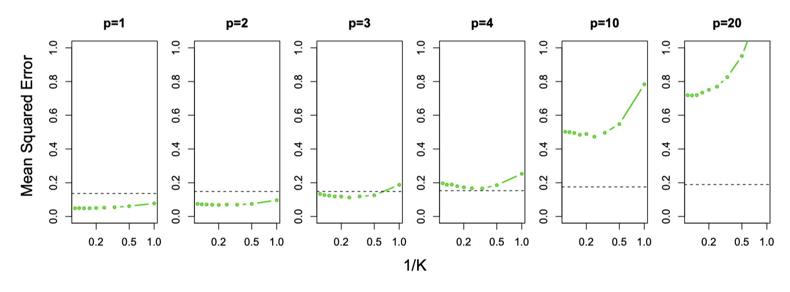
![FIGURE 2.7. A simulation example, demonstrating the curse of dimensionality and its effect on MSE, bias and variance. The input features are uniformly distributed in [−1, 1]^p for p = 1,…, 10 The top left panel shows the target function (no noise) in \mathbb{R}: f(X) = e^{−8||X||^2}, and demonstrates the error that 1-nearest neighbor makes in estimating f(0). The training point is indicated by the blue tick mark. The top right panel illustrates why the radius of the 1-nearest neighborhood increases with dimension p. The lower left panel shows the average radius of the 1-nearest neighborhoods. The lower-right panel shows the MSE, squared bias and variance curves as a function of dimension p.](images/ESLII-fig2-7.png)