Intro to Data Science
  • Home
  • Introduction
    • Overview
    • Two Cultures
    • Causal Inference
  • Python Basics
    • Python Setup
    • NumPy & pandas
    • Data Inspection
    • Subsetting
  • EDA
    • Visualize
    • Explore
    • Wrangling
  • Linear Models
    • Model Basics
    • Implementations
    • Regression Analysis
  • ML Basics
    • Introduction
    • Regularization
    • Implementations
    • K-Nearest Neighbors
  • Classification
    • Logistic Regression
    • Generative Models
  • Trees

On this page

  • Generalized Linear Models
  • Logistic Regression
    • Emperical probability/ Odds
    • Prediction Values
    • Predictive Accuracy
      • Evaluation of predicted probability
      • Evaluation of predicted class
      • 분류모형의 성능을 평가하기 위한 여러 지표들
      • 종합: 모형평가
    • Decision Boundary
  • Basis Functions
  • Neural Network/Deep Learning
  • Multiclass (K > 2)
    • Blowdown data
    • MNIST digits data
  • Other Model Families

Logistic Regression

Mixed

Author

Sungkyun Cho

Published

June 11, 2026

Load packages
# numerical calculation & data frames
import numpy as np
import pandas as pd

# visualization
import matplotlib.pyplot as plt
import seaborn as sns
import seaborn.objects as so

# statistics
import statsmodels.api as sm

# pandas options
pd.set_option('mode.copy_on_write', True)  # pandas 2.0
pd.options.display.float_format = '{:.2f}'.format  # pd.reset_option('display.float_format')
pd.options.display.max_rows = 7  # max number of rows to display

# NumPy options
np.set_printoptions(precision = 2, suppress=True)  # suppress scientific notation

# For high resolution display
import matplotlib_inline
matplotlib_inline.backend_inline.set_matplotlib_formats("retina")

Generalized Linear Models

Ordinary least squares (OLS)

  • Mean function: \(E(Y | X = x_i) = \beta_0 + \beta_1 x_i\)
  • Distribution: \((Y | X = x_i) \sim N(\beta_0 + \beta_1 x_i, \sigma^2)\)

Source: p.107, Applied Regression Analysis and Generalized Linear Models (3e), by John Fox

Generalized linear models (GLM)

OLS의 가정에 맞지 않는 경우, 가정을 완화한 모델

  • Mean function: \(E(Y | X = x_i) = f(\beta_0 + \beta_1 x_i)\)
  • Distribution: \((Y | X = x_i) \sim \text{Exponential family}\)

Binary outcome: Logistic regression

  • Mean function: \(\displaystyle E(Y | X = x_i) = f(\beta_0 + \beta_1 x_i)\),   \(\displaystyle f = \frac{1}{1 + e^{-x}}\) : sigmoid function
  • Distribution: \((Y | X = x_i) \sim \text{Bernoulli}(p_i)\): n=1인 이항분포

Count outcome: Poisson regression

  • Mean function: \(\displaystyle E(Y | X = x_i) = f(\beta_0 + \beta_1 x_i)\),   \(\displaystyle f = e^x\)
  • Distribution: \((Y | X = x_i) \sim \text{Poisson}(\lambda_i)\)

전형적으로 나타나는 \(X\)와 \(Y\)의 관계

Logistic Regression

Response 변수가 binary로 두 개의 클래스에 속하는 경우; \(Y \in \{C_1, C_2\}\)
보통 관심이 있는 쪽을 1로, 나머지를 0으로 코딩하여 전개

예제: Blowdown
p.274, Applied Linear Regression (4e) by Sanford Weisberg

Data: blowdown2.csv

1999년 7월 4일, 미네소타 북동부의 바운더리 워터스 카누 지역 야생지대에 시속 90마일이 넘는 폭풍이 몰아쳐 숲에 심각한 피해를 입혔습니다. Rich 등(2007)은 이 지역에 대한 매우 광범위한 지상 조사를 통해 이 폭풍의 영향을 연구하여 3600여 그루의 나무의 생사 여부를 확인했습니다.

d: 나무의 지름(cm),  y: 나무가 죽은 경우 1, 그렇지 않으면 0
spp: 나무의 종,  s: 특정 지역의 폭풍의 심각도

blowdown = pd.read_csv('data/blowdown2.csv')

# black spruce에 제한
blowbs = blowdown.query('spp == "black spruce"')
blowbs
         d    s  y           spp  log2d
17    9.00 0.02  0  black spruce   3.17
24   11.00 0.03  0  black spruce   3.46
25    9.00 0.03  0  black spruce   3.17
...    ...  ... ..           ...    ...
3646  9.00 0.94  1  black spruce   3.17
3647 17.00 0.94  1  black spruce   4.09
3661  8.00 0.98  1  black spruce   3.00

[659 rows x 5 columns]

기존의 ordinary least squares (OLS) 방법으로 fit을 하면, (linear probability model)

  • Y; 1: event, 0: non-event
  • Mean funtion \(E(Y | X = x_i)\)을 생각하면 각 나무의 두께에 해당하는 쓰러진 나무의 비율, 즉 확률값으로 해석할 수 있음.
code
(
    so.Plot(blowbs, x='log2d', y='y')
    .add(so.Dots(alpha=.3), so.Jitter(y=.1))
    .add(so.Line(), so.PolyFit(1))
    .limit(y=(-0.2, 1.2))
    .scale(y=so.Continuous().tick(at=[0, 1]))
    .layout(size=(6, 3.5))
    .label(x='Log Diameter (cm)', y='Died vs. Survived', title="Linear Fit")
).show()

(
    nsplot(blowbs, x='log2d', y='y', alpha=0, df_n=6)
    .add(so.Dots(alpha=.3), so.Jitter(y=.1))
    .limit(y=(-0.2, 1.2))
    .scale(y=so.Continuous().tick(at=[0, 1]))
    .layout(size=(6, 3.5))
    .label(x='Log Diameter (cm)', y='Died vs. Survived', title="Nonlinear Fit")
).show()

Conditional distribution (근방에서)

code
(
    blowbs.query('d < 15')
    .assign(log2d = blowbs['log2d'].round(1))
    .pipe(so.Plot, x='y')
    .add(so.Bar(), so.Hist(stat="proportion", common_norm=False))
    .facet("log2d", wrap=5)
    .layout(size=(8, 4))
    .label(title='log d = {}'.format)
)

Emperical probability/ Odds

이제 y를 직접 예측하기보다, 확률을 예측하는 방식을 취하면,

  • 각 두께를 가진 나무들의 개수 (m)와
  • 그 중에 태풍으로 죽은 나무의 수 (died)를 고려하면,
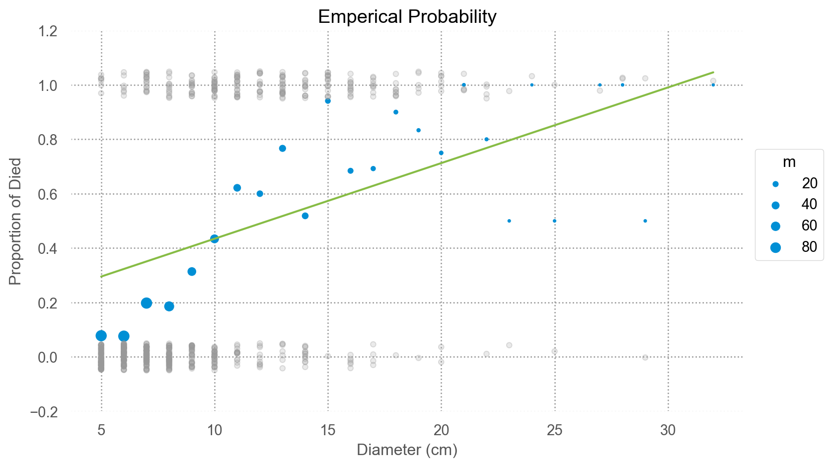
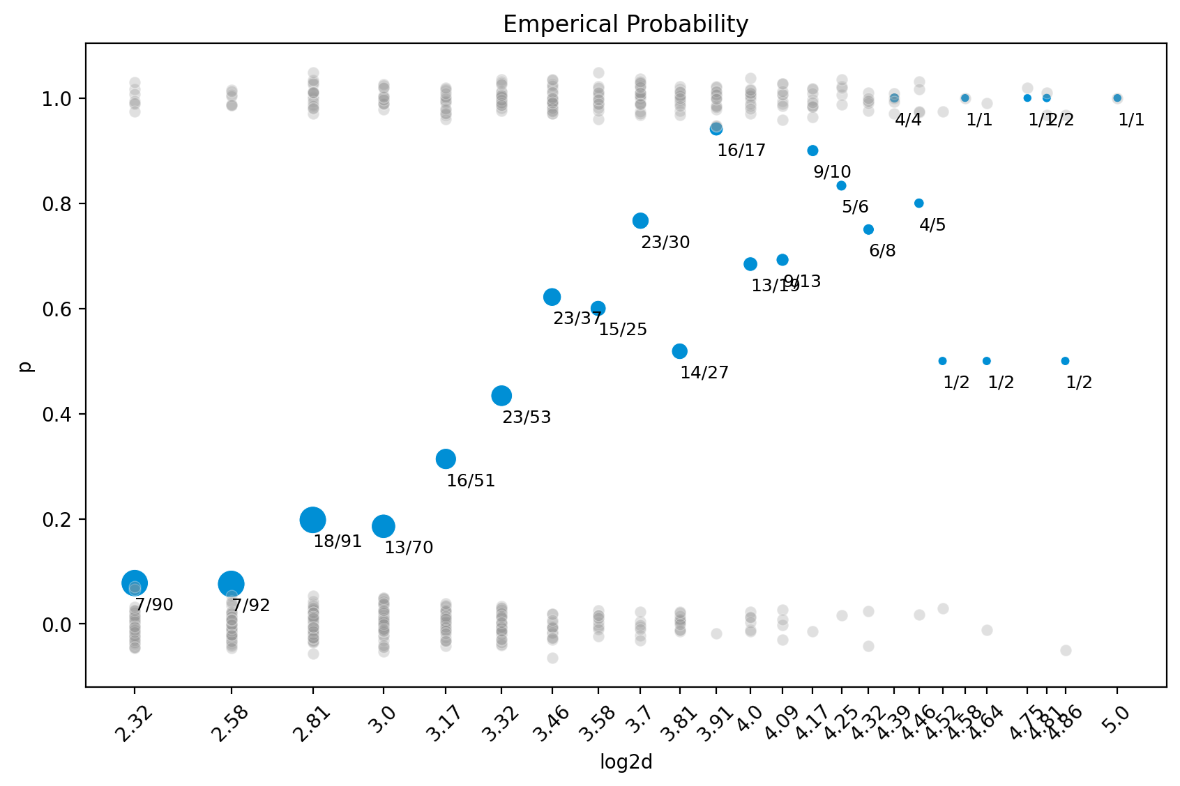
  • 나무의 두께에 따라 죽은 나무 수의 비율 (p= died/m)을 계산할 수 있음. 이를 emperical probability라고 함.
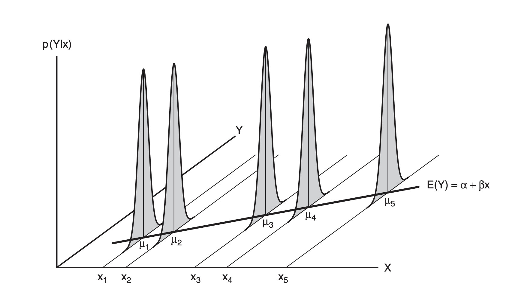
  • 사실, 이 p는 binary response (0, 1)의 conditional mean(평균)인데,
  • 통계적으로 표현하면 \(E(Y|d=d_i)\)이며 선형모형의 mean function를 제공.
blowbs_bn = blowbs.groupby("d")["y"].agg([("died", "sum"), ("m", "count"), ("p", "mean")]).reset_index()
blowbs_bn
       d  died   m    p
0   5.00     7  90 0.08
1   6.00     7  92 0.08
2   7.00    18  91 0.20
..   ...   ...  ..  ...
22 28.00     2   2 1.00
23 29.00     1   2 0.50
24 32.00     1   1 1.00

[25 rows x 4 columns]
code
(
    so.Plot(blowbs_bn, x='d', y='p')
    .add(so.Dot(), pointsize='m')
    .add(so.Dots(alpha=.3, color=".6"), so.Jitter(y=.1), x=blowbs.d, y=blowbs.y)
    # .add(so.Line(), so.PolyFit(5))
    .add(so.Line(color="#87bc45"), so.PolyFit(1))
    .limit(y=(-0.2, 1.2))
    .layout(size=(8, 5))
    .label(title='Emperical Probability', y = 'Proportion of Died', x='Diameter (cm)')
)

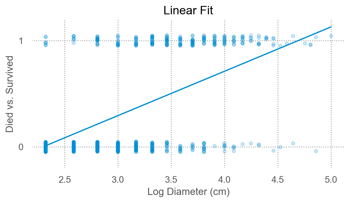
  • OLS estimate으로도 충분한가?
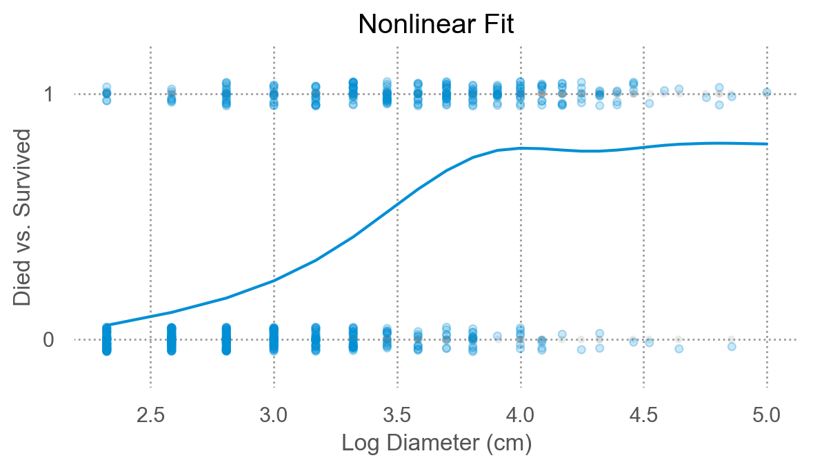
  • 1차보다는 고차 다항함수로 fit한다면?

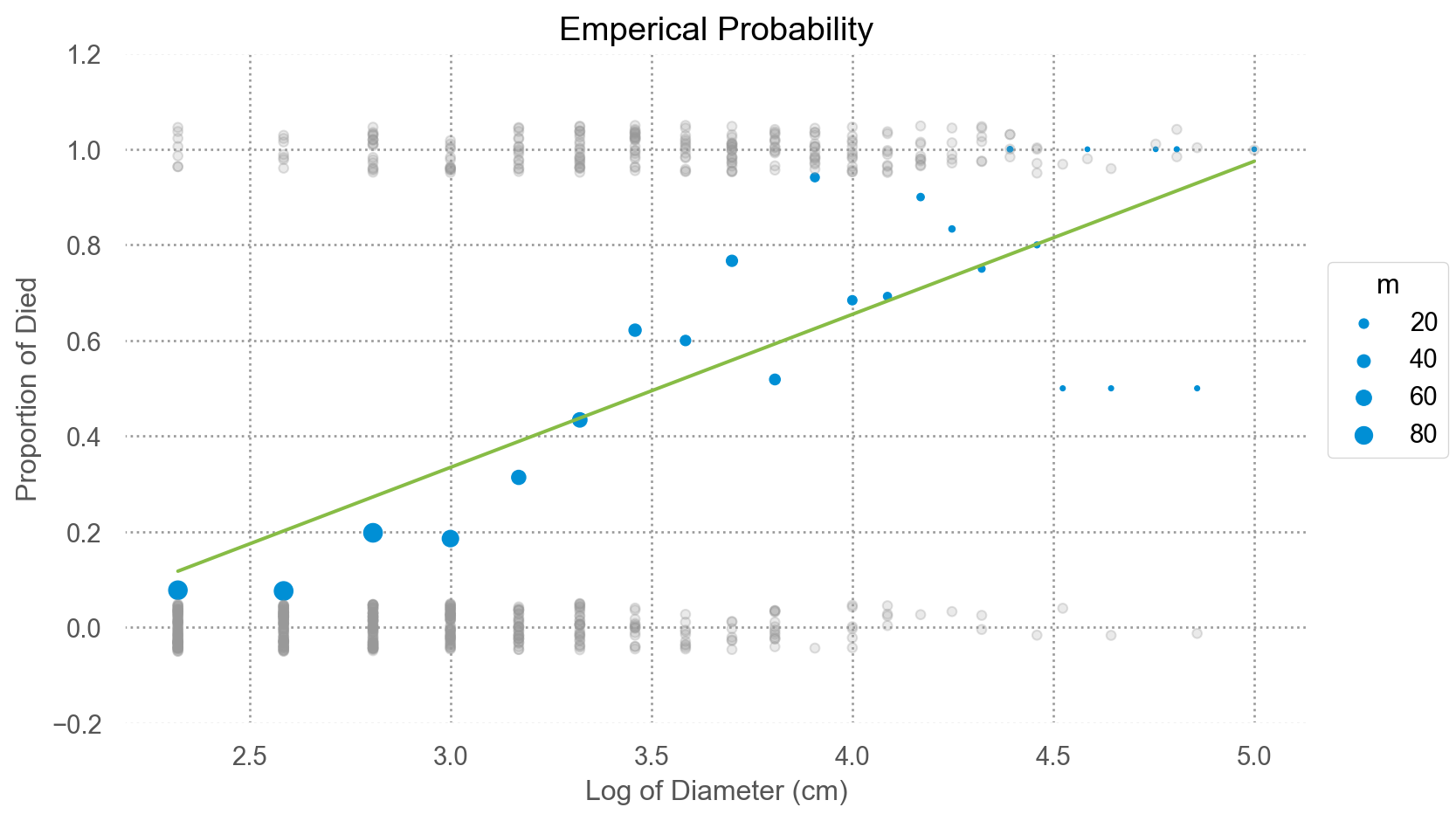
우선 d를 log2 변환해서 살펴보면,

code
blowbs_bn["log2d"] = np.log2(blowbs_bn["d"])
(
    so.Plot(blowbs_bn, x='log2d', y='p')
    .add(so.Dot(), pointsize='m')
    .add(so.Dots(alpha=.3, color=".6"), so.Jitter(y=.1), x=blowbs.log2d, y=blowbs.y)
    .add(so.Line(color="#87bc45"), so.PolyFit(1))
    .limit(y=(-0.2, 1.2))
    .layout(size=(8, 5))
    .label(title='Emperical Probability', y = 'Proportion of Died', x='Log of Diameter (cm)')
)

위에서 살펴본 OLS의 문제들 즉,

  • 잔차에 패턴이 보인다는 것은 충분히 좋은 모형이 아니라는 것을 의미하고,
  • 예측값이 확률을 의미하지 못할 수 있음.
  • 잔차의 분포도 Gaussian과는 거리가 멈.

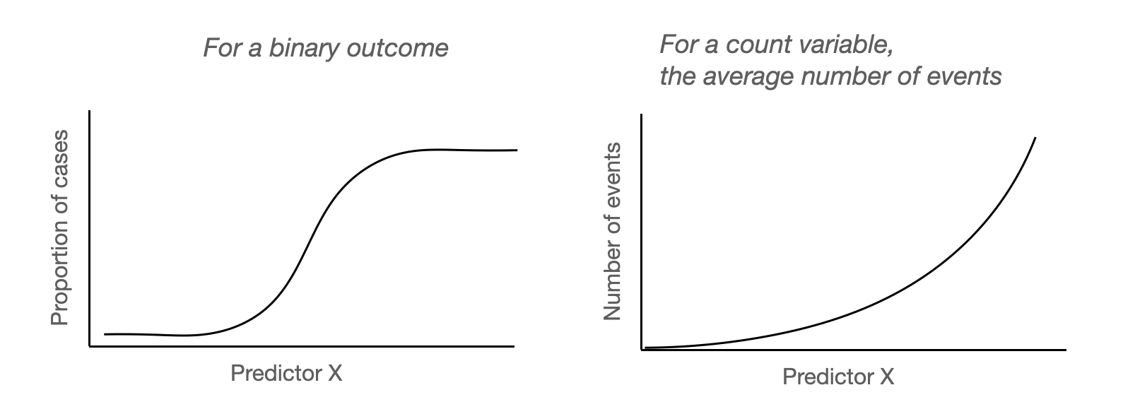
이런 문제들을 해결하고 예측값이 분명한 “확률”의 의미를 품도록 여러 방식이 제시되는데 주로 사용되는 것이 logistic regression임.

Important

Binary outcome을 예측하는 logistic regression 모형은 binary 값을 예측하는 것이 아니고, 확률 값을 예측하는 것임.
이후에 이를 이용해 binary outcome을 예측.

  • 예를 들어, 두께가 5cm인 (특정 종의) 나무가 태풍에 쓰러질 확률(true probability)을 파악하고자 함.
  • 이 때, 관측값은 5cm인 나무 중 쓰러진 나무의 “비율”이고, 이 관측치들로부터 true probability를 추정하고자 함.
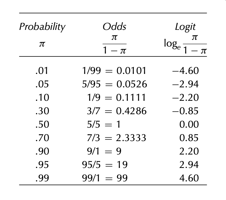
Odds의 정의: 실패할 확률 대비 성공할 확률의 비율

\(\displaystyle odds = \frac{P(Y = 1)}{P(Y = 0)} = \frac{p}{1-p}\)

예를 들어, 5cm 두께의 나무는 90그루 중 7그루가 죽었으므로 83그루는 살았음.
즉, 죽음:생존 = 7:83 = 대략 1:12 - 1 그루 죽을 때 12 그루는 생존했음; 생존 가능성이 12배 높음.
혹은 분수로 표현하며 odds = 7/83 = 0.084; 1000 그루가 살았다면 84 그루는 죽었음.
확률값(\(p= \frac{7}{90}\))을 이용해 계산하면, \(\displaystyle odds = \frac{\frac{7}{90}}{1 - \frac{7}{90}} = \frac{7}{90-7} = \frac{7}{83}\)

확률과 odds, logit(log odds)의 관계

blowbs_bn = blowbs_bn.assign(odds = lambda x: x.p / (1 - x.p))
# p = 1인 경우 odds가 무한대가 되므로 편의상 inf 값을 50으로 대체
blowbs_bn["odds"] = blowbs_bn["odds"].apply(lambda x: 50 if x == np.inf else x)
blowbs_bn
       d  died   m    p  log2d  odds
0   5.00     7  90 0.08   2.32  0.08
1   6.00     7  92 0.08   2.58  0.08
2   7.00    18  91 0.20   2.81  0.25
..   ...   ...  ..  ...    ...   ...
22 28.00     2   2 1.00   4.81 50.00
23 29.00     1   2 0.50   4.86  1.00
24 32.00     1   1 1.00   5.00 50.00

[25 rows x 6 columns]

이 odds를 선형모형으로 나무두께로 예측하려고 하는 것인데, 예를 들어,

\(\widehat{odds} = b_0 + b_1 \cdot \log_{2} d\)

odds 값의 범위는 (0, \(\infty\))이므로, 선형모형으로 fit하는 것이 적절하지 않음.
한편, odds를 log 변환하면, 그 범위는 (\(-\infty\), \(\infty\))가 되어 선형모형으로 fit하는 것이 적절해짐.

이 때, 예측모형은 log odds가 \(x\)에 대해 선형적으로 연결된다고 가정하는 것임. 즉,

\(\displaystyle \log \widehat{odds} = \log\left(\frac{\hat{p}}{1-\hat{p}}\right) = b_0 + b_1 \cdot \log_{2} d\)
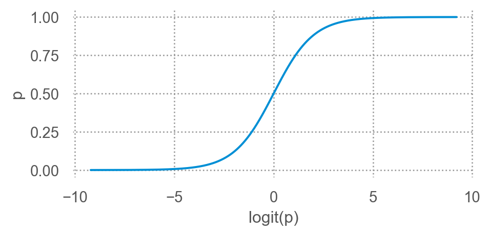
이를 logit 함수로 간단히 표현하면; 전통적 통계에서 선호
\(\displaystyle logit(\hat p) = b_0 + b_1 \cdot \log_{2} d\),   \(\displaystyle logit(x) := \log\left(\frac{x}{1-x}\right)\)

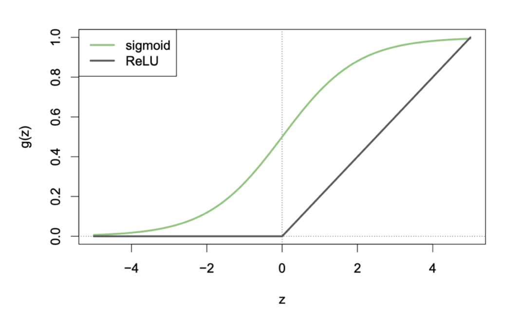
logit의 역함수인 sigmoid 함수로 표현하면; machine learning에서 선호
\(\displaystyle \hat p = \sigma(b_0 + b_1 \cdot \log_{2} d)\),   \(\displaystyle \sigma(x) := \frac{1}{1 + e^{-x}}\)

이를 확률로 표현하면,
\(\displaystyle P(Y=1|X=x) = E(Y|X=x) = \sigma(b_0 + b_1 \cdot \log_{2} d)\)

즉, logit은 예측변수 \(x\) 와 선형적으로 연결되는데 반해, 확률 \(p\) 는 예측변수 \(x\) 와 비선형적 관계를 맺음

Note

Mean function \(E(Y|X)\)을 변형하는 방식으로 표현할 때,

\(f(E(Y|X))=\beta_0 + \beta_1 X_1 + \cdots + \beta_n X_n\)

  • 이 때, \(f\)를 link function이라고 하고,
  • 여기서는 logit 함수를 link function으로 사용함.

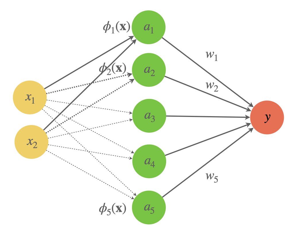
Machine learning에서는, 그 역함수를 이용해 선형함수 쪽을 변형해 다음과 같이 표현하는데,

\(E(Y|X)=f(\beta_0 + \beta_1 X_1 + \cdots + \beta_n X_n)\)

  • 이 때, \(f\)를 activation function이라고 부름.
  • 여기서는 sigmoid 함수를 activation function으로 사용함.

sigmoid 함수는 logisitic 함수라고도 부름.
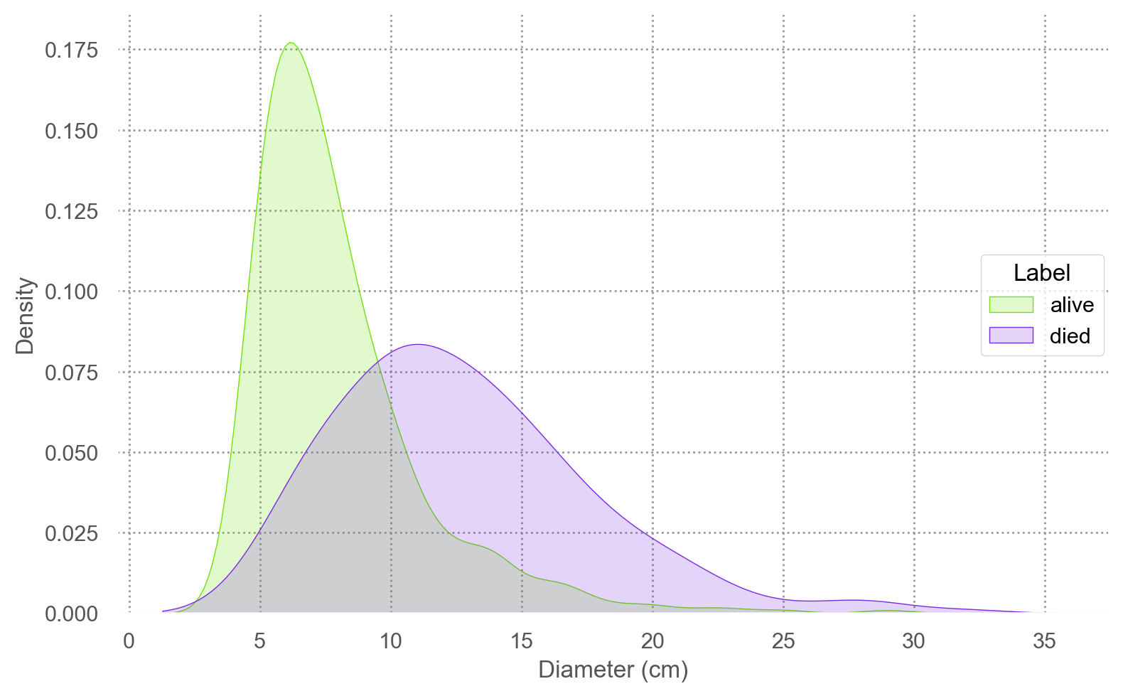
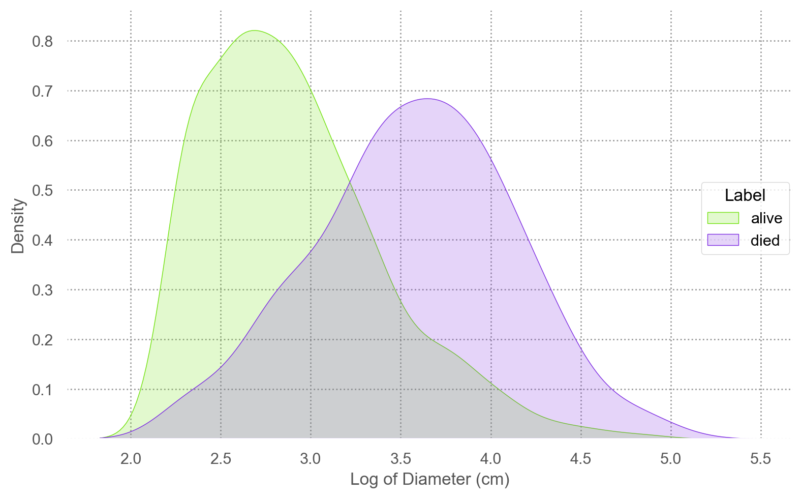
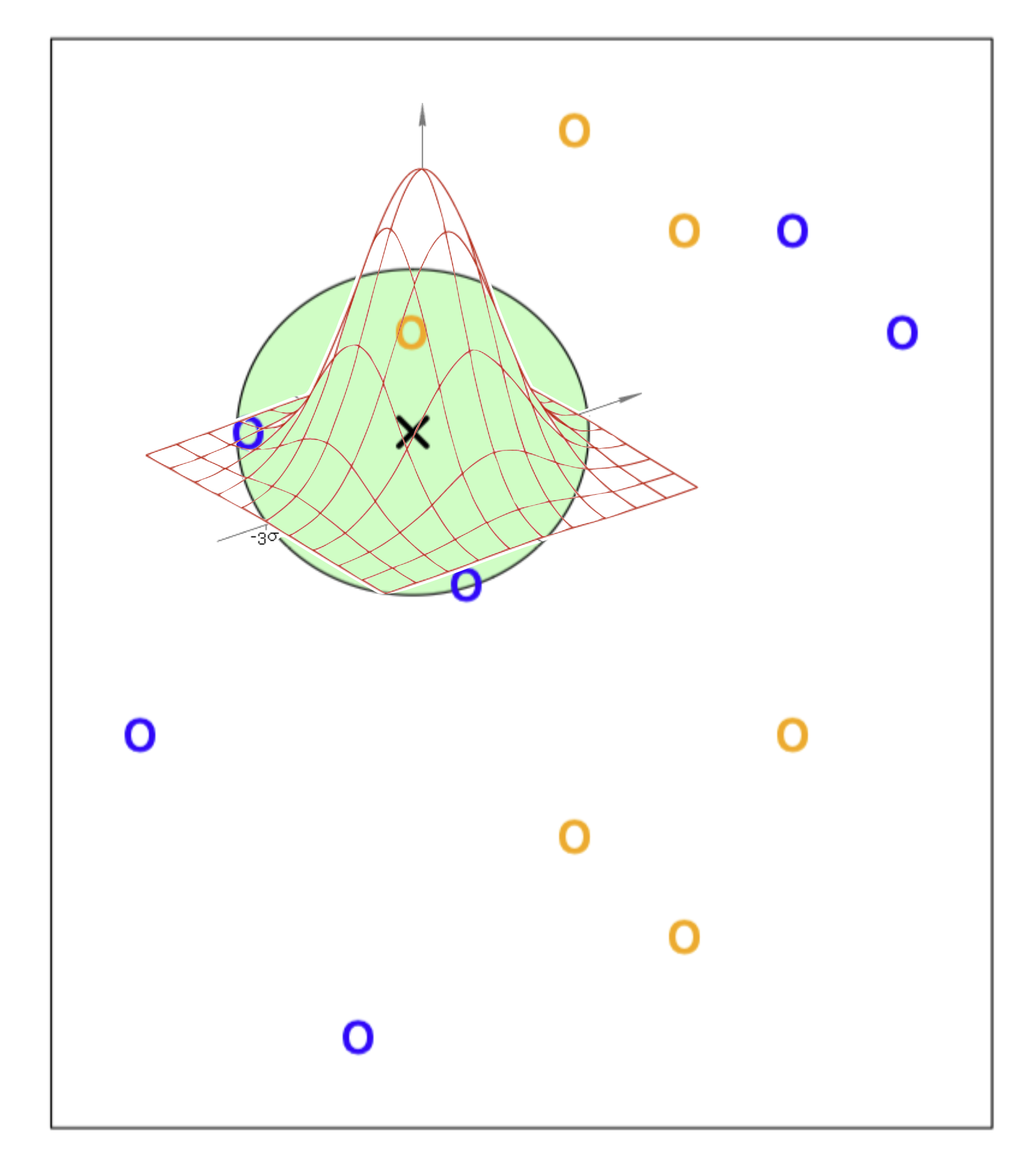
한편, 각 클래스 내에서 \(X\)가 multivariate Gaussian 분포를 따르고, 이 분포의 covariance matrix가 (모든 클래스에서) 동일하다고 가정하면 (즉, 모든 클래스에서 분산과 공분산이 같으면),
log odds가 \(X\)에 대해 선형적으로 연결된다는 것을 보일 수 있음: 즉, log odds를 선형함수로 모델링해도 되는 충분조건을 제공해줌.

  • 여기서는 쓰러진 나무와 산 나무의 두께가 Gaussian 분포를 따르고,
  • 그 두 분포의 분산이 동일하다면(변수가 1개이므로 공분산/상관계수는 없음), log odds가 \(X\)에 대해 선형적 연결될 수 있음.
  • 나무의 두께(d)를 log2 변환한 이유임 (오른쪽 그림)
code
blowbs["label"] = blowbs["y"].map({0: "alive", 1: "died"})
(
    so.Plot(blowbs, x='d', color='label')
    .add(so.Area(), so.KDE(common_norm=False))
    #.scale(color=so.Nominal())
    .scale(color=['#70e20c', '#7d2be2'])
    .layout(size=(8, 5))
    .label(x="Diameter (cm)", y="Density", color="Label")
).show()

(
    so.Plot(blowbs, x='log2d', color='label')
    .add(so.Area(), so.KDE(common_norm=False))
    .scale(color=['#70e20c', '#7d2be2'])
    .layout(size=(8, 5))
    .label(x="Log of Diameter (cm)", y="Density", color="Label")
).show()

이제, log odds을 구해, \(X\)에 대해 선형적인 패턴이 있는지 확인해보면,

blowbs_bn = blowbs_bn.assign(log_odds = lambda x: np.log(x.odds))
blowbs_bn   
       d  died   m    p  log2d  odds  log_odds
0   5.00     7  90 0.08   2.32  0.08     -2.47
1   6.00     7  92 0.08   2.58  0.08     -2.50
2   7.00    18  91 0.20   2.81  0.25     -1.40
..   ...   ...  ..  ...    ...   ...       ...
22 28.00     2   2 1.00   4.81 50.00      3.91
23 29.00     1   2 0.50   4.86  1.00      0.00
24 32.00     1   1 1.00   5.00 50.00      3.91

[25 rows x 7 columns]
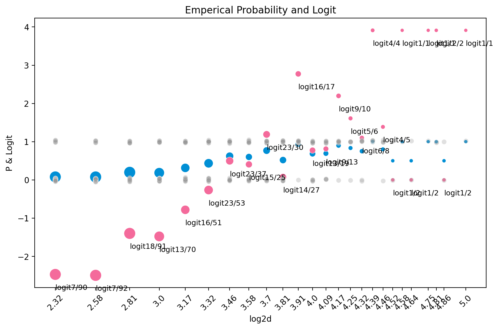
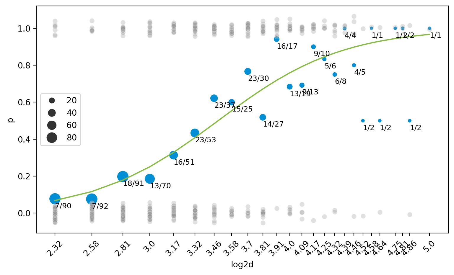
관측값들과 emperical probability와 log odds을 함께 살펴보면,

code
fig, ax = plt.subplots(1, 1, figsize=(10, 6))

sns.scatterplot(x=blowbs_bn.log2d, y=blowbs_bn.p, size=blowbs_bn.m, c="#008fd5", sizes=(20, 200), ax=ax)

def jitter(values, j):
    return values + np.random.normal(0, j, values.shape)

sns.scatterplot(x=blowbs.log2d, y=jitter(blowbs.y, 0.02), alpha=.3, c=".6", ax=ax)

for i, row in blowbs_bn.iterrows():
    ax.annotate(f"{row.died:n}/{row.m:n}", xy=(row.log2d, row.p), xytext=(row.log2d, row.p-0.05), size=9)

ax.set_xticks(blowbs_bn.log2d.unique())
ax.set_xticklabels(blowbs_bn.log2d.unique().round(2))
ax.tick_params(axis='x', rotation=45)
ax.set_title("Emperical Probability")
ax.legend_.remove()

Logit 값(분홍색)을 추가해서 그리면,

code
fig, ax = plt.subplots(1, 1, figsize=(10, 6))

sns.scatterplot(x=blowbs_bn.log2d, y=blowbs_bn.p, size=blowbs_bn.m, sizes=(20, 200), c="#008fd5", ax=ax, legend=False)

sns.scatterplot(x=blowbs_bn.log2d, y=blowbs_bn.log_odds, size=blowbs_bn.m, sizes=(20, 200), color="#f46a9b", ax=ax)
def jitter(values, j):
    return values + np.random.normal(0, j, values.shape)

sns.scatterplot(x=blowbs.log2d, y=jitter(blowbs.y, 0.02), alpha=.3, c=".6", ax=ax)

for i, row in blowbs_bn.iterrows():
    ax.annotate(f"logit{row.died:n}/{row.m:n}", xy=(row.log2d, row.log_odds), xytext=(row.log2d, row.log_odds-0.4), size=9)

ax.set_xticks(blowbs_bn.log2d.unique())
ax.set_xticklabels(blowbs_bn.log2d.unique().round(2))
ax.tick_params(axis='x', rotation=45)
ax.set_ylabel("P & Logit")
ax.set_title("Emperical Probability and Logit")
ax.legend_.remove()

# # polyfit 5
# x = np.linspace(blowbs_bn.log2d.min(), blowbs_bn.log2d.max(), 100)
# y = np.polyval(np.polyfit(blowbs_bn.log2d, blowbs_bn.log_odds, 5), x)
# sns.lineplot(x=x, y=y, ax=ax, color=".6")

# # polyfit 1
# y = np.polyval(np.polyfit(blowbs_bn.log2d, blowbs_bn.log_odds, 1), x)
# sns.lineplot(x=x, y=y, ax=ax, color=".6")

위의 logit값을 선형모형으로 예측하는 모형: \(\displaystyle \log\left(\frac{\hat{p}}{1-\hat{p}}\right) = b_0 + b_1 \cdot \log_{2} d\)

파라미터 \(b_0, b_1\)의 추정은 잔차들의 제곱의 합을 최소로 하는 OLS 방식은 부적절하며, 대신에 Maximum Likelihood Estimation을 사용함.

  • 아이디어는 관측치가 전체적으로 관찰될 likelihood가 최대가 되도록 \(b_0, b_1\)을 선택하는 것임
  • 이를 위해서 적절한 확률모형을 결합시켜야 함.
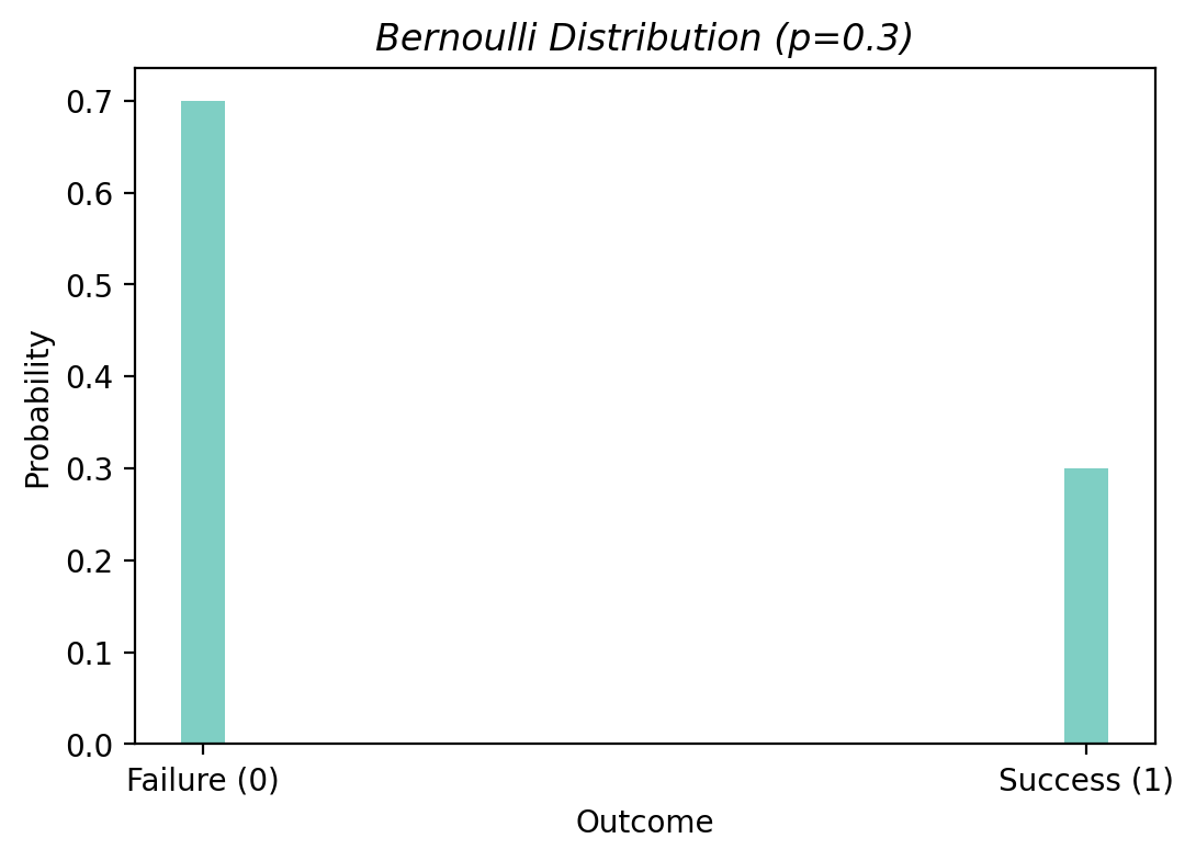
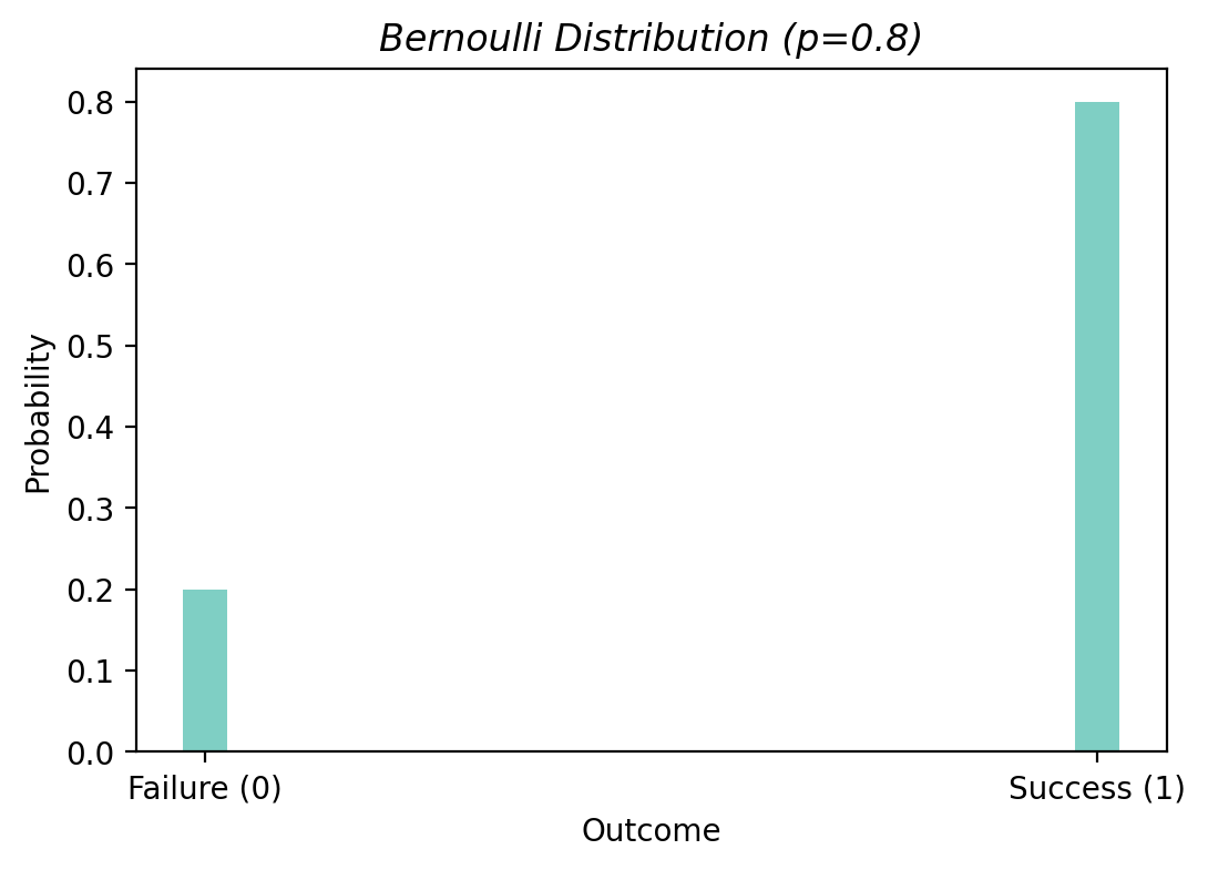
  • 선택하는 확률 모형은 Bernoulli 분포임; 평균 \(E(Y|X) = p\)이고, \(logit(E(Y|X)) = b_0 + b_1 \cdot \log_{2} d\)
    • Y를 1의 발생 빈도수로 변환해 Binomial distribution (이항분포)로 전개하는 방식도 있음; binomial logit model
  • 관찰값은 Bernoulli 분포로부터 발생했다고 가정함으로써, 실제 관찰값들이 관찰될 확률/가능도를 기준으로 파라미터를 추정할 수 있음.


blowbs.sort_values("log2d")
         d    s  y           spp  log2d  label
2102  5.00 0.45  0  black spruce   2.32  alive
724   5.00 0.18  0  black spruce   2.32  alive
723   5.00 0.18  1  black spruce   2.32   died
...    ...  ... ..           ...    ...    ...
1784 29.00 0.38  1  black spruce   4.86   died
1079 29.00 0.25  0  black spruce   4.86  alive
3455 32.00 0.80  1  black spruce   5.00   died

[659 rows x 6 columns]
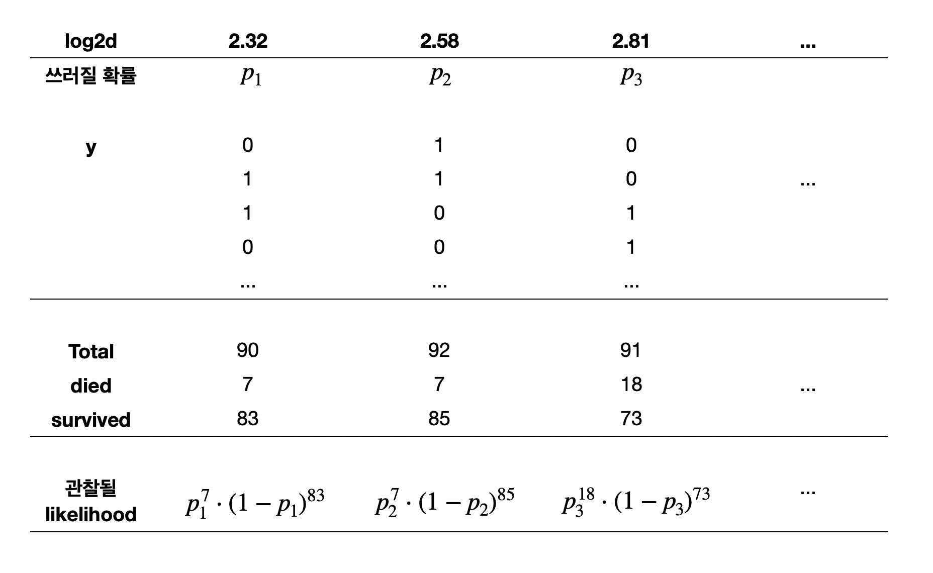
각 likelihood는 관측치들이 모두 독립적으로 발생했다고 가정했을 때의 확률값이고,
각 \(x_i\)(그에 대응하는 \(p_i\))에 대해 관측치(\(y_i\))가 관찰된 확률은 간결하게 다음과 같이 표현할 수 있음.

\[p_i^{y_i} (1-p_i)^{1-y_i}\]

\[\displaystyle \text{log likelihood}=\log \prod_{i=1}^{n}{P_i}=\sum_{i=1}^{n} y_i \cdot \log p_i + (1-y_i) \cdot \log(1-p_i)\]

모든 데이터가 관찰될 likelihood = \(p_1^7 (1-p_1)^{83} \cdot p_2^7 (1-p_2)^{85} \cdot p_3^{18} \cdot (1-p_3)^{73} \cdots\)

이 때, 모형을 예측변수 \(X\)의 1차 다항함수로 fit한다면,   \(\displaystyle \log\left(\frac{p_i}{1-p_i}\right) = \beta_0 + \beta_1 \cdot x_i\) 인데,
변형하면   \(\displaystyle p_i = \sigma(\beta_0 + \beta_1 x_i) = \frac{1}{1+e^{-(\beta_0 + \beta_1 \cdot x_i)}}\)

Likelihood = \(\displaystyle \left(\frac{1}{1+e^{-(\beta_0 + \beta_1 \cdot 2.32)}}\right)^7 \left(1 - \frac{1}{1+e^{-(\beta_0 + \beta_1 \cdot 2.32)}}\right)^{83} \cdot \left(\frac{1}{1+e^{-(\beta_0 + \beta_1 \cdot 2.58)}}\right)^7 \left(1 - \frac{1}{1+e^{-(\beta_0 + \beta_1 \cdot 2.58)}}\right)^{85} \cdots\)

이 Likelihood가 최대가 되도록 \(\beta_0, \beta_1\)의 추정치를 찾음.

손실함수 vs. 가능도

위의 Log likelihood = \(\displaystyle \sum_{i=1}^{n} y_i \cdot \log p_i + (1-y_i) \cdot \log(1-p_i)\)는

머신러닝에서 손실함수로 사용되는 cross-entropy loss와 (거의) 동일함.

\(L = -\frac{1}{n} \sum_{i=1}^{n} y_i \cdot \log p_i + (1-y_i) \cdot \log (1-p_i)\)

= [cross-entropy]: \(H(\tilde{q}, p)\): [실제값(y)를 \(p\)의 분포로 잘못 모델링했을 때의 평균 정보량]

= [부정확하게 예측되어 발생하는 정보 손실량: Kullback-Leibler divergence] + [경험분포 자체의 평균 정보량]

= \(KL(\tilde{q} | p) + H(\tilde{q})\)

관측 데이터로부터 경험분포 \(\tilde{q}\)와, 모델이 만드는 모델분포 \(p\)를 구분

분포 \(y=1\)일 때 \(y=0\)일 때
경험분포 \(\tilde{q}\): 여기서는 degenerate Bernoulli 분포 \(y_i\) (관측값) \(1 - y_i\)
모델분포 \(p\) \(\hat{p}_i\) (예측값) \(1 - \hat{p}_i\)
정보량
  • 정보량: \(-\log p\)
  • 엔트로피 \(H\): 평균 정보량(정보의 기대값) \(\displaystyle \sum p \cdot (-\log p) = \sum -p \cdot \log p\)

By Claude Sonnet 4.6

오늘 길에서 만나는 사람들의 키를 예측한다고 했을 때, 키가 180cm가 넘는 여자를 만나는 사건의 정보:

상황 설정

오늘 서울 길거리를 걷습니다. 마주치는 사람들의 키는 서울 여성의 실제 분포 \(p\)를 따릅니다. 이 \(p\)는 내가 어떻게 생각하든 상관없이 세상에 고정되어 있는 실제 빈도입니다.

사건 — 가능성이 하나로 확정되는 순간

걷기 전에는 “165cm일 수도 있고, 170cm일 수도 있고, 2m가 넘을 수도 있다”는 가능성들이 열려 있습니다. 누군가를 마주치는 순간, 그 가능성들 중 하나가 실현됩니다. “키 180cm 이상 여성을 만났다”는 그 실현된 하나의 사건입니다.

정보량 — 실현된 사건이 얼마나 드문가/놀라운가

\[I(\text{180cm 이상}) = -\log_2 p(\text{180cm 이상}) = -\log_2 (0.001) \approx 10 \text{ bits}\]

여기서 \(p\)는 서울에서 실제로 180cm 이상 여성이 얼마나 드문가입니다. 이 사건이 실제 세계에서 0.1%밖에 일어나지 않는다는 사실 자체가 정보량을 결정합니다.

엔트로피 — 걷기 전, 실제 세계의 불확실성

\[H(p) = \sum_x p(x) \cdot (-\log_2 p(x))\]

집을 나서기 전 상태입니다. 오늘 어떤 키의 사람을 만날지 모릅니다. 이 불확실성의 총량이 엔트로피입니다.

엔트로피는 정보량의 가중평균입니다. 자주 만나는 사람(높은 \(p\), 낮은 정보량)과 드물게 만나는 사람(낮은 \(p\), 높은 정보량)을 모두 고려해서 평균 낸 것입니다.

세 개념의 시점과 역할

개념 시점 역할
사건 마주친 순간 가능성 중 하나가 실현됨
정보량 \(I(x)\) 마주친 후 이 사건이 실제로 얼마나 드문가/놀라운가
엔트로피 \(H(p)\) 걷기 전 실제 세계의 평균 불확실성
Regularization

앞서 Ridge, Lasso에서와 비슷한 원리로 OLS가 아닌 ML(maximum likelihood) estimator에 penalty를 적용하는 방식임.
즉, likeihood에 대한 계산에서 penalty term을 추가함

에를 들어, Logistic regression with L2 regularization: 다음 손실함수를 최소화하도록 파라미터를 추정

\(\displaystyle L = \frac{1}{n} \left[ - \sum_{i=1}^{n} \left(y_i \cdot \log p_i + (1-y_i) \cdot \log(1-p_i)\right) + \frac{\lambda}{2} \sum_{j=1}^{p} \beta_j^2 \right]\)

import statsmodels.formula.api as smf

mod = smf.logit('y ~ log2d', data=blowbs).fit()
print(mod.summary())
Optimization terminated successfully.
         Current function value: 0.499165
         Iterations 6
                           Logit Regression Results                           
==============================================================================
Dep. Variable:                      y   No. Observations:                  659
Model:                          Logit   Df Residuals:                      657
Method:                           MLE   Df Model:                            1
Date:                Tue, 27 May 2025   Pseudo R-squ.:                  0.2316
Time:                        23:59:25   Log-Likelihood:                -328.95
converged:                       True   LL-Null:                       -428.10
Covariance Type:            nonrobust   LLR p-value:                 4.888e-45
==============================================================================
                 coef    std err          z      P>|z|      [0.025      0.975]
------------------------------------------------------------------------------
Intercept     -7.8162      0.628    -12.437      0.000      -9.048      -6.584
log2d          2.2408      0.190     11.773      0.000       1.868       2.614
==============================================================================
Scikit-learn implementation

Scikit-learn의 LogisticRegression()은 디폴트로 \(l2\) regularization을 사용함: 참고 문서

우선, train-test split을 통해 데이터를 나눈 후, LogisticRegression()을 적용하면,

from sklearn.model_selection import train_test_split
from sklearn.linear_model import LogisticRegression

X = blowbs[['log2d']]
y = blowbs['y']

X_train, X_test, y_train, y_test = train_test_split(X, y, test_size=0.5, random_state=0)

lr = LogisticRegression(penalty=None)  # l1, l2 regularization 가능
lr.fit(X_train, y_train)

print(lr.coef_, lr.intercept_)
# [[2.08]] [-7.26]

# As a DataFrame with column names
coefs = pd.DataFrame({"coef": lr.coef_[0], "name": X.columns})
coefs
#    coef   name
# 0  2.08  log2d

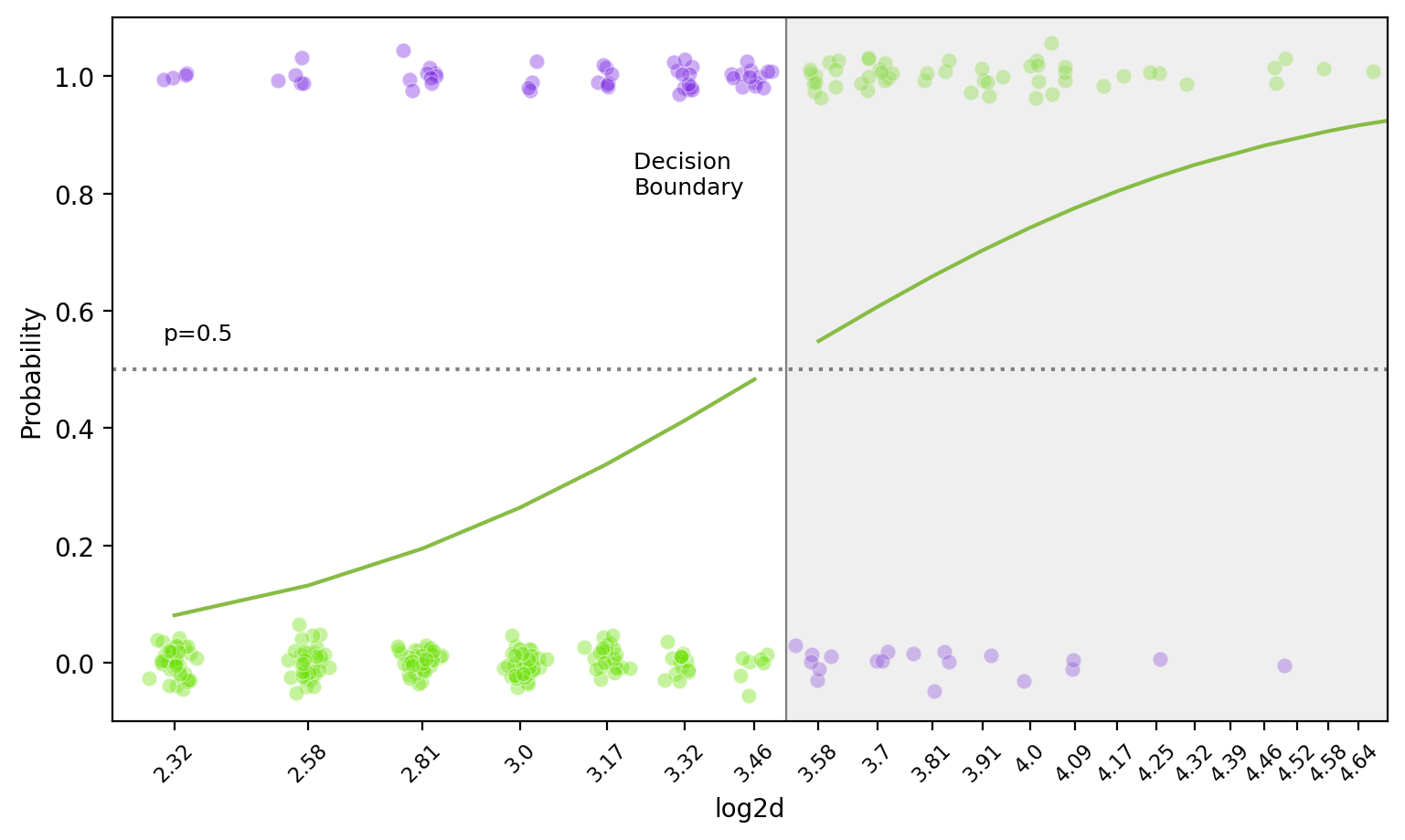
위 fitted model의 예측값들

code
fig, ax = plt.subplots(1, 1, figsize=(9, 5))

sns.scatterplot(x=blowbs_bn.log2d, y=blowbs_bn.p, size=blowbs_bn.m, c="#008fd5", sizes=(20, 200), ax=ax)

def jitter(values, j):
    return values + np.random.normal(0, j, values.shape)

sns.scatterplot(x=blowbs.log2d, y=jitter(blowbs.y, 0.02), alpha=.3, c=".6", ax=ax)

for i, row in blowbs_bn.iterrows():
    ax.annotate(f"{row.died:n}/{row.m:n}", xy=(row.log2d, row.p), xytext=(row.log2d, row.p-0.05), size=9)

ax.set_xticks(blowbs_bn.log2d.unique())
ax.set_xticklabels(blowbs_bn.log2d.unique().round(2))
# x-axis with 45 degree rotation
ax.tick_params(axis='x', rotation=45)

# fitted line
sns.lineplot(x=blowbs.log2d, y=mod.predict(blowbs["log2d"]), ax=ax, color="#87bc45")

plt.show()

Prediction Values

예측값

Logistic regression에서는 세 가지 타입의 예측값들이 있음.

  • Predicted probability:   \(\displaystyle \hat{p} = \frac{1}{1+e^{-(b_0 + b_1 \cdot x)}}\)
  • Odds:   \(\displaystyle odds = \frac{\hat{p}}{1 - \hat{p}} = e^{b_0 + b_1 \cdot x}\),  Odds ratio:   \(\displaystyle \frac{odds_1}{odds_2} = e^{b_1 \cdot (x_1 - x_2)}\)
  • Log odds:   \(\displaystyle logit = b_0 + b_1 \cdot x\)

이 확률값을 이용해 binary outcome인 클래스를 예측할 수 있음.

# using statsmodels package, not scikit-learn
blowbs_pred = blowbs.assign(
    pred_prob = mod.predict(blowbs["log2d"]),
    pred_odds = lambda x: x.pred_prob / (1 - x.pred_prob),
    pred_logit = lambda x: mod.predict(blowbs["log2d"], which="linear")
)
blowbs_pred.iloc[:, 1:]
        s  y           spp  log2d  label  pred_prob  pred_odds  pred_logit
17   0.02  0  black spruce   3.17  alive       0.33       0.49       -0.71
24   0.03  0  black spruce   3.46  alive       0.48       0.94       -0.06
25   0.03  0  black spruce   3.17  alive       0.33       0.49       -0.71
...   ... ..           ...    ...    ...        ...        ...         ...
3646 0.94  1  black spruce   3.17   died       0.33       0.49       -0.71
3647 0.94  1  black spruce   4.09   died       0.79       3.83        1.34
3661 0.98  1  black spruce   3.00   died       0.25       0.33       -1.09

[659 rows x 8 columns]

예를 들어, 두께(log2d)가 3인 나무의 경우,

  • Probabiliy: 태풍에 쓰러질 확률은 25%로 예측되며,
  • Odds: 태풍에 쓰러지지 않을 가능성 대비 쓰러질 가능성의 비율은 1:0.33이므로 대략 3:1로 예측됨. 즉 다시 말하면, 1 그루가 쓰러진다면 3 그루는 쓰러지지 않을 것으로 예측함.
    • Odds가 1이면 event의 확률(p)이 0.5
    • Odds가 1보다 작으면 event의 확률(p)이 0.5보다 작고,
    • Odds가 1보다 크면 event의 확률(p)이 0.5보다 큼.
  • Log odds (logit): 확률 p의 [0, 1]의 값을 무한한 값으로 늘려 linearly fit할 수 있게 함.
모형의 파라미터 해석

Odds의 비율 (odds ratio, OR)을 통해 해석

  • \(\displaystyle odds: \frac{\hat{p}}{1 - \hat{p}} = e^{b_0 + b_1 \cdot x}=e^{b_0}\cdot e^{b_1 \cdot x}\)  로부터

  • \(x\)가 1 증가할 때 odds의 비율: \(\displaystyle odds ~ratio: \frac{\frac{\hat{p_2}}{1 - \hat{p_2}}}{\frac{\hat{p_1}}{1 - \hat{p_1}}} = e^{b_1 \cdot (x+1) - b_1 \cdot x} = e^{b_1}\)

  • 즉, \(x\)가 1 증가하면, odds가 “몇 배”로 증가하는지를 나타냄.

  • 따라서, odds ratio가 1보다 크면 (\(b_1\)이 양수) \(x\)가 1 증가할 때, event의 odds가 커지며,

  • odds ratio가 1보다 작으면 (\(b_1\)이 음수) event의 odds가 줄어듬.

위의 경우, \(\displaystyle \widehat{odds} = e^{-7.82 + 2.24 \cdot log_2(d)}\) 이므로 odds ratio = \(e^{2.24} = 9.4\)

  • 해석하면, 나무의 두께가 (log2 scale로) 1 늘어남 (2배 증가)에 따라 태풍에 나무가 쓰러질 odds가 9.4배 증가함
  • 다시 말하면, 나무의 두께가 (log2 scale로) 1 늘어남 (2배 증가)에 따라 태풍에 나무가 쓰러지지 않을 가능성 대비 쓰러질 가능성이 9.4배 증가함.
  • 나무의 두께 (원래 d)로 말하면, 두께가 10% 두꺼워지면, \(e^{2.24 \cdot log_2(1.1)}=1.36\) 배, 즉 odds가 36% 증가함.

\(b_0\): d = 1일 때의 odds이므로 \(\displaystyle e^{-7.82 + 2.34 \cdot 0} = e^{-7.82} = 0.004\), 즉 두께가 1cm 일 때 태풍에 나무가 쓰러지지 않을 가능성 대비 쓰러질 가능성은 0.004임.

Scikit-learn implementation

Scikit-learn의 LogisticRegression()은 디폴트로 \(l2\) regularization을 사용함: 참고 문서

from sklearn.model_selection import train_test_split
from sklearn.linear_model import LogisticRegression

X = blowbs[['log2d']]
y = blowbs['y']

X_train, X_test, y_train, y_test = train_test_split(X, y, test_size=0.5, random_state=0)

lr = LogisticRegression(penalty=None)  # l1, l2 regularization 가능
lr.fit(X_train, y_train)

# predict_proba: 각 클래스에 대한 확률을 반환
# predict: 예측된 클래스를 반환 (threshold=0.5)
test_pred = X_test.assign(
    y=y_test,
    pred_prob=lr.predict_proba(X_test)[:, 1],  # 확률값
    pred_class=lr.predict(X_test),  # 클래스
    pred_odds=lambda x: x.pred_prob / (1 - x.pred_prob),  # odds
    pred_logit=lambda x: np.log(x.pred_odds),  # log odds
)
test_pred.head(5)

#       log2d  y  pred_prob  pred_class  pred_odds  pred_logit
# 2890   3.46  1       0.48           0       0.94       -0.07
# 574    3.81  0       0.66           1       1.93        0.66
# 96     3.17  0       0.34           0       0.51       -0.67
# 2773   3.46  1       0.48           0       0.94       -0.07
# 1813   3.58  1       0.55           1       1.21        0.19

Predictive Accuracy

모형의 예측 정확성

분류 문제의 경우, 보통 두 단계를 거쳐 예측

  • Inference: 클래스에 속할 확률을 추정; 확률을 추정하지 않는 알고리즘도 있음.
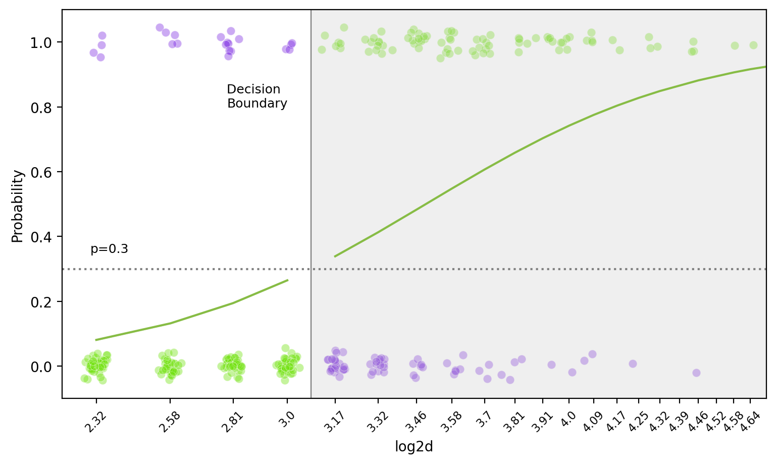
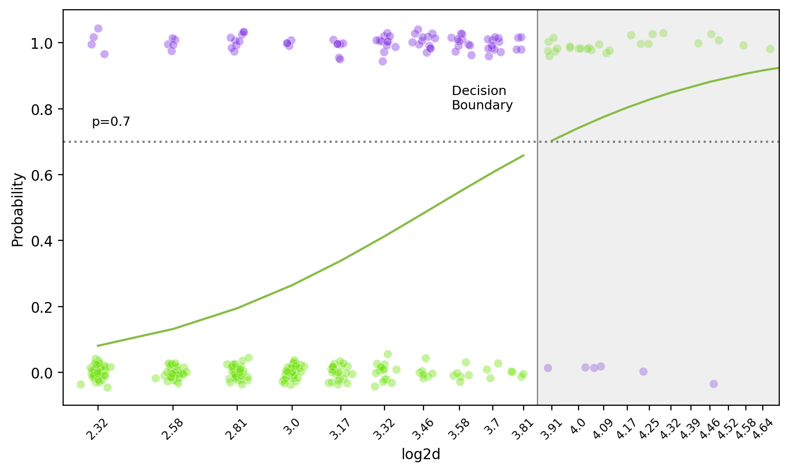
  • Decision: 추정된 확률을 기반으로 클래스를 결정
    • 기본적으로 0.5 이상이면 1로, 그렇지 않으면 0으로 분류
    • Threshold를 조정해 분류를 조정할 수 있음
      • 예를 들어, 확실한 경우(p > 0.8)에만 1로 분류
    • 애매한 확률 구간의 경우 결정을 유보할 수 있음; reject option

이 때, 모형의 예측 정확성을 평가하는 두 가지 방식이 있음.

  • 확률 대한 예측 정확성 (evaluating predicted probability)
  • 클래스에 대한 예측 정확성 (evaluating predicted class)

Evaluation of predicted probability

Deviance Residuals

이제 이 모형이 좋은 모형인지 살펴보기 위해 residual, 잔차를 살펴볼 수 있는가?

  • Pearson residual: \(\displaystyle \frac{y_i - \hat{p}_i}{\sqrt{\hat{p}_i (1-\hat{p}_i)}}\)
  • Deviance residual: \(\displaystyle sign(y_i - \hat{p}_i) \sqrt{-2[y_i \log\hat{p}_i + (1-y_i) \log(1-\hat{p}_i)]}\)

Deviance를 이용해 OLS에서의 \(R^2\)와 비슷한 개념을 구성: Pseudo R-squared

Model deviance, \(D = -2[\log likelihood - \log likelihood_{\text{perfect}})]\)

  • Perfect model의 likelihood: 1
  • Null deviance: 절편만 있는 모형의 deviance; 856.2073760911842
  • Pseudo R-squared: \(\displaystyle \frac{Null~Deviance - Deviance}{Null~Deviance}\)
  • Cox-Snell’s Pseudo R-squared
  • Nagelkerke’s Pseudo R-squared

“Coefficient of discrimination” (Tjur, 2009): average \(\hat{p}\) when \(y=1\) - average \(\hat{p}\) when \(y=0\)

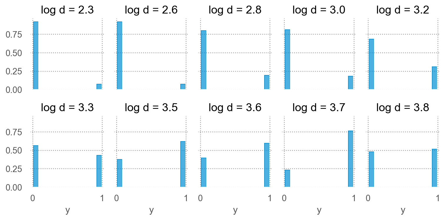
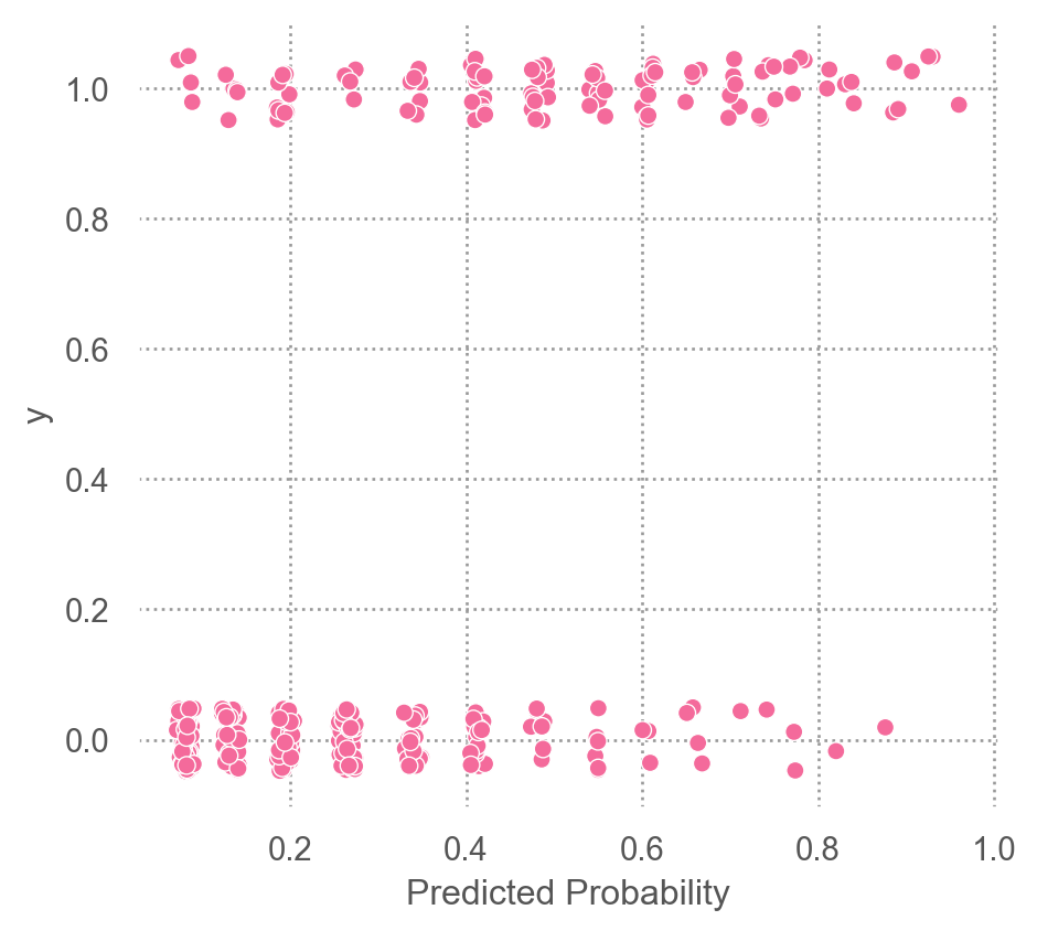
클래스별 예측 확률의 분포/히스토그램

code
test_pred["y2"] = test_pred["y"].map({0: "survived (y=0)", 1: "died (y=1)"})
(
    so.Plot(test_pred, x='pred_prob')
    .add(so.Bars(color="#ef9b20"), so.Hist(bins=12))
    .facet("y2")
    .label(x="Predicted Probability", y="Count")
    .layout(size=(7, 4))
)

각 (확률 값의) bin에 포함되는 관측치의 실제 값(\(y \in \{0, 1\}\))의 비율을 계산해 시각화

code
from sklearn.calibration import calibration_curve

# 3. calibration_curve로 실제 비율 계산
prob_true, prob_pred = calibration_curve(
    test_pred["y"], test_pred["pred_prob"], n_bins=10, strategy="uniform"
)

(
    so.Plot(x=prob_pred, y=prob_true)
    .add(so.Line(marker="o", color="#f46a9b"))
    .add(so.Line(color=".3", linestyle=":"), y=prob_pred)
    .scale(x=so.Continuous().tick(at=np.linspace(0, 1, 11)))
    .label(
        x="(10-Binned) Predicted Probability",
        y="Observed Event Percentage\n(Emperical Probability)",
        title="Calibration Plot",
    )
    .layout(size=(5, 4.5))
)

Evaluation of predicted class

Important

예측된 확률을 기반으로 binary outcome/class으로 예측하여, 모형의 예측력을 평가

  • 예측된 확률값에 대해 임계치를 정하여, 예를 들어 0.5보다 크면 1, 0.5보다 작으면 0으로 분류하여, 이 binary 예측값과 실제값을 비교하여, 예측력을 평가
  • Confusion matrix
  • ROC curve

Threshold: 0.5인 경우, accuracy rate: 0.78

Predicted Truth
survied(0) died(1)
survied(0) 203 54
died(1) 19 54


Predicted Truth
survied(0) died(1)
survied(0) True Negative False Positive
died(1) False Negative True Positive

다른 threshold를 적용하면,

Threshold: 0.1인 경우,

Predicted Truth
survied(0) died(1)
survied(0) 42 4
died(1) 180 104

Accuracy rate: 0.44


Threshold: 0.9인 경우

Predicted Truth
survied(0) died(1)
survied(0) 222 104
died(1) 0 4

Accuracy rate: 0.68


code
from sklearn.metrics import accuracy_score
from ISLP import confusion_table

# cutoff = 0.5
cm = confusion_table(test_pred["pred_class"], test_pred["y"])
score = accuracy_score(test_pred["y"], test_pred["pred_class"])

display(cm)
print(f"Accuracy rate: {score:.2f}")

# cutoff = 0.1
cm = confusion_table(test_pred["pred_prob"] > 0.1, test_pred["y"])
score = accuracy_score(test_pred["y"], test_pred["pred_prob"] > 0.1)

display(cm)
print(f"Accuracy rate: {score:.2f}")

# cutoff = 0.9
cm = confusion_table(test_pred["pred_prob"] > 0.9, test_pred["y"])
score = accuracy_score(test_pred["y"], test_pred["pred_prob"] > 0.9)

display(cm)
print(f"Accuracy rate: {score:.2f}")

분류모형의 성능을 평가하기 위한 여러 지표들

Precision & Recall: 정보 검색 시스템의 탐색 능력을 평가하는데에서 유래

  • Precision (정밀도): \(\hat{y}=1\)일 때, \(y=1\)일 확률
    • 정보검색에서 반환된 문서들 중 실제로 관련 있는 문서의 비율
      • 높은 precision은 사용자가 검색 결과에서 불필요한 정보를 적게 얻고, 대부분 유용한 정보를 얻는다는 것을 의미
      • 하지만, 관련은 있지만 놓친 정보는 많을 수 있음.
      • 검색 결과의 정확도를 평가
    • 시스템이 스팸으로 분류한 이메일 중 실제 스팸인 이메일의 비율
      • 높은 precision은 스팸으로 잘못 분류된 정상 이메일이 적다는 것을 의미
      • 하지만, 스팸 이메일이 정상 이메일함에 나타날 수 있음.
    • 검사를 통해 암으로 진단받은 사람이 실제로 암을 가지고 있을 확률
      • 높은 precision은 암 진단을 받은 사람에게 잘못된 암 진단을 내리지 않는 것을 의미
  • Recall (재현율): \(y=1\)일 때, \(\hat{y}=1\)일 확률
    • 정보검색에서 관련 문서들 중에서 실제로 시스템이 반환한 문서의 비율
      • 높은 recall은 사용자가 찾고자 하는 모든 관련 정보를 검색 결과에서 얻을 수 있다는 것을 의미
      • 하지만, 관련 없는 정보도 많이 포함될 수 있음.
      • 검색 시스템의 탐색 능력을 평가
    • 실제 스팸 이메일 중에서 시스템이 스팸으로 올바르게 분류한 비율
      • 높은 recall은 대부분의 스팸 이메일이 정확히 스팸으로 분류된다는 것을 의미
      • 하지만, 정상 이메일이 스팸함으로 분류될 수 있음.
    • 실제로 암을 가진 사람 중에서 검사를 통해 암으로 진단받은 사람의 비율
      • 높은 recall은 암 환자를 놓치지 않고 모두 찾아낸다는 것을 의미
    • 참 양성, true positive rate (TPR), 또는 sensitivity라고도 함

precision & recall trade-off: 이 둘 사이에는 종종 상충 관계가 있음. Precision을 높이기 위해 예측 확률에 대한 더 엄격한 기준을 사용하면 recall이 낮아질 수 있고, 반대로 recall을 높이기 위해 더 느슨한 기준을 사용하면 precision이 낮아질 수 있음.

  • 정보 검색의 맥락: precision을 높여 사용자가 불필요한 정보를 받지 않게 해주며, recall을 높여 필요한 정보를 놓치지 않도록 함.

  • 스팸 필터링의 맥락: precision을 높여 자주 스팸 메일함을 확인하지 않아도 되도록 하며, recall을 높여 대부분의 스팸 이메일이 차단되어 정상 메일함에서 보이지 않도록 쾌적한 환경을 제공할 수 있음.

Sensitivity & specificity: 의학 분야에서 진단 테스트의 정확성을 평가하는데에서 유래
Precision & recall이 주로 양성(positive) 클래스에 초점을 두는 반면, sensitivity & specificity는 양성(positive)와 음성(negative) 클래스 모두에 초점을 둠.

한편, 이상치 탐지라든가 희귀 질병 진단 등 클래스 불균형 데이터셋에서는 precision & recall이 더 유용할 수 있음.

  • Sensitivity (민감도): \(y=1\)일 때, \(\hat{y}=1\)일 확률
    • True positive rate (TPR) (= Recall)
    • 높은 민감도는 질병이 있는 사람을 놓치지 않고 모두 찾아내는 것(참 양성)을 의미
  • Specificity (특이도): \(y=0\)일 때, \(\hat{y}=0\)일 확률
    • True negative rate (TNR)
    • 실제로 질병이 없는 사람을 얼마나 잘 (질병이 없다고) 식별하는지(참 음성)를 나타냄
    • Specific의 의미는 초점이 되는 특정(specific) 질병에만 반응하는 진단 툴이기를 바란다는 의미임. 가령, 폐렴이 아닌데(아마도 다른 병일 수 있는데) 폐렴이라고 진단하지 않기를 기대함.
    • 높은 특이도는 (특정) 질병이 없는 사람에게 그 질병이 있다고 잘못 진단하지 않는 것을 의미함
      • 단, 희귀 질병을 진단하는 경우, 정상인(negative)을 올바로 식별하는 것은 매우 쉽기 때문에 질병이 없는 사람에 대한 판별력이 과대추정될 수 있음; precision이 더 유용할 수 있음.
    • 1 - FPR (False Positive Rate; false alarm)
    • 0, 1을 바꿨을 때의 즉, 0을 (양성)기준으로 했을 때의 recall 값이 됨.
    • 특이도가 높은 테스트라면 질병이 없다는 판정은 신뢰할 만함. 즉, 0(음성)을 기준으로한 sensitivity가 높은 것이 됨.

거짓 음성 비율: False negative rate (FNR); \(y=1\)일 때, \(\hat{y}=0\)일 확률: 1 - sensitivity
- 정상이라고 진단된 환자가 실제로 암인 확률

거짓 양성 비율: False positive rate (FPR) 또는 False alarm; \(y=0\)일 때, \(\hat{y}=1\)일 확률: 1 - specificity
- 정상인 사람이 검사를 통해 암으로 진단받을 확률

위의 confusion matrix로부터 지표들을 계산하면,

Threshold: 0.1인 경우,

Predicted Truth
survied(0) died(1)
survied(0) 42 4
died(1) 180 104


Threshold: 0.9인 경우

Predicted Truth
survied(0) died(1)
survied(0) 222 104
died(1) 0 4
  • recall = 104 / (4 + 104) = 0.96
  • precision = 104 / (180 + 104) = 0.37
  • specificity = 42 / (42 + 180) = 0.19
  • accuracy = (42 + 104) / (42 + 4 + 180 + 104) = 0.44


  • recall = 4 / (4 + 104) = 0.04
  • precision = 4 / (0 + 4) = 1.00
  • specificity = 222 / (222 + 0) = 1.00
  • accuracy = (222 + 4) / (222 + 104 + 0 + 4) = 0.68

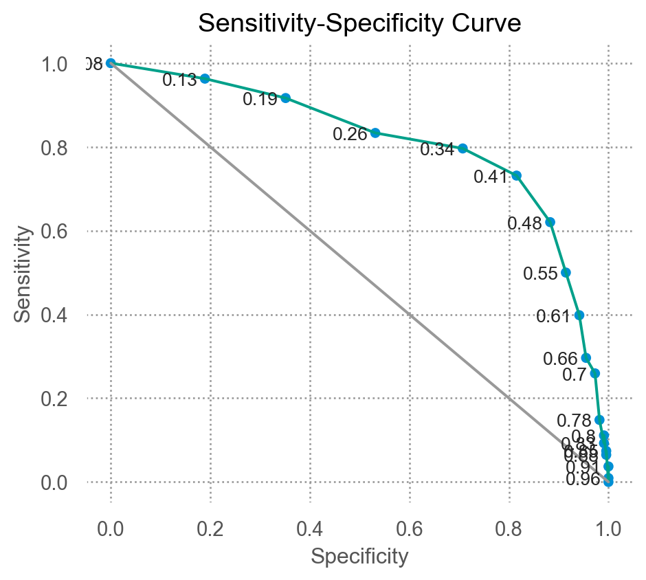
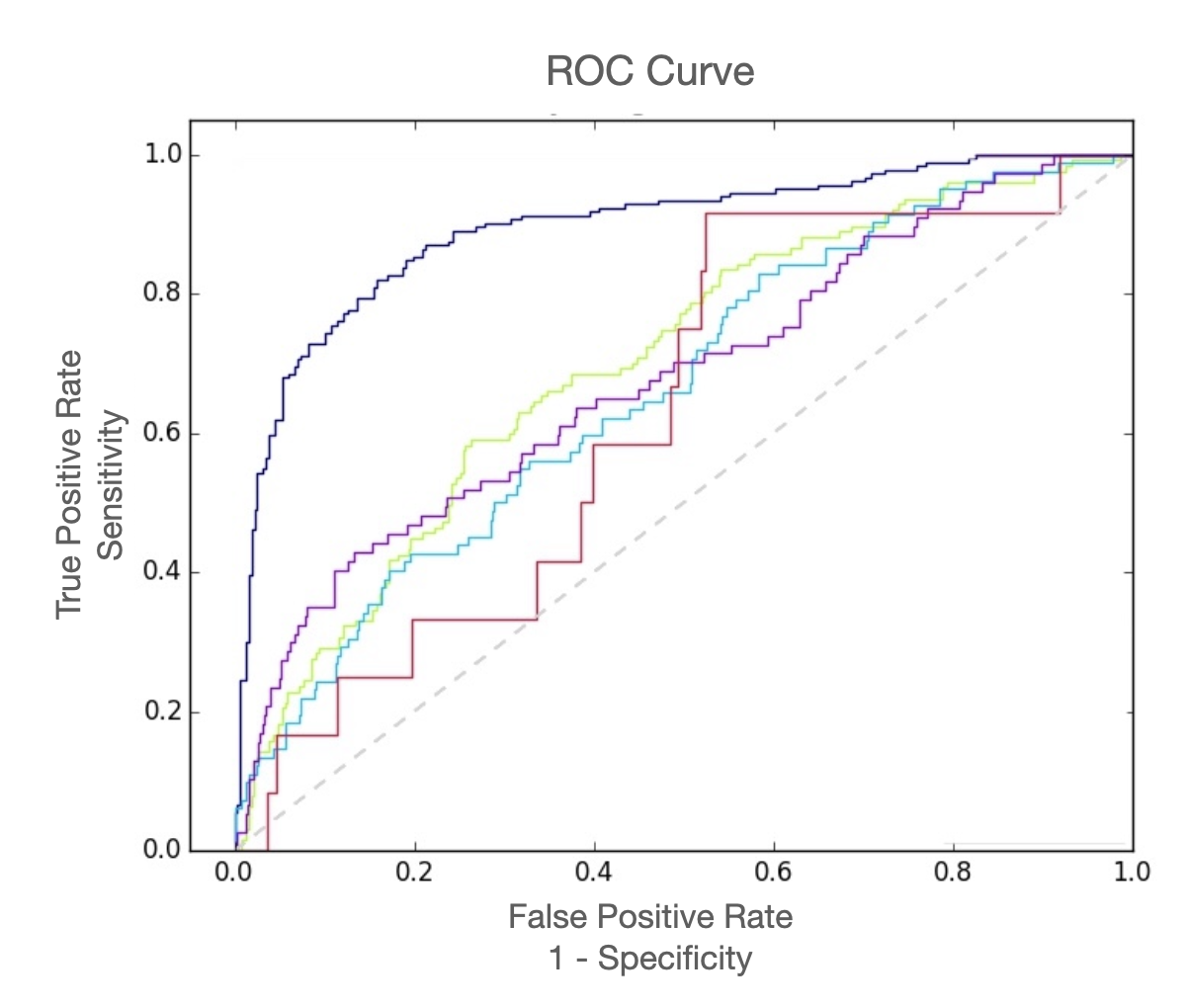
Receiver operating characteristic (ROC) curve

예측된 확률에 대한 임계치를 조정함에 따라 옳은 예측과 틀린 예측의 비율이 어떻게 달라지는지 살펴봄으로써 임계치를 설정하는데 도움을 줌

잘못된 예측에 대한 비용이 다르다면, 특정 임계치를 선택하는 것을 고려해야 함

code
from sklearn.metrics import roc_curve

fpr, tpr, thresholds = roc_curve(test_pred.y, test_pred.pred_prob)
roc = pd.DataFrame(
    {
        "thresholds": thresholds.round(2),
        "False Pos": fpr,
        "sensitivity(TPR)": tpr,
        "specificity(TNR)": 1 - fpr
    }
)
roc.sort_values("thresholds").head(10)

## ROC curve
# 위에서 얻은 roc 데이터을 사용하여 그리거나
# RocCurveDisplay를 이용
from sklearn.metrics import RocCurveDisplay
roc_display = RocCurveDisplay(fpr=fpr, tpr=tpr).plot()

# scikit-learn의 visualization 문서 참조
# https://scikit-learn.org/stable/visualizations.html

code
from sklearn.metrics import precision_recall_curve

precision, recall, thresholds = precision_recall_curve(test_pred.y, 
test_pred.pred_prob)
pr = pd.DataFrame(
    {
        "thresholds": np.append(thresholds.round(2), 1),
        "precision": precision,
        "recall": recall,
        "f1-score": 2 * precision * recall / (precision + recall)
    }
).query("recall > 0.1")
pr.sort_values("thresholds").head(10)

# precision-recall curve
# 위에서 얻은 pr 데이터을 사용하여 그리거나
# PrecisionRecallDisplay를 이용
from sklearn.metrics import PrecisionRecallDisplay
pr_display = PrecisionRecallDisplay(precision=precision, recall=recall).plot()

# scikit-learn의 visualization 문서 참조
# https://scikit-learn.org/stable/visualizations.html

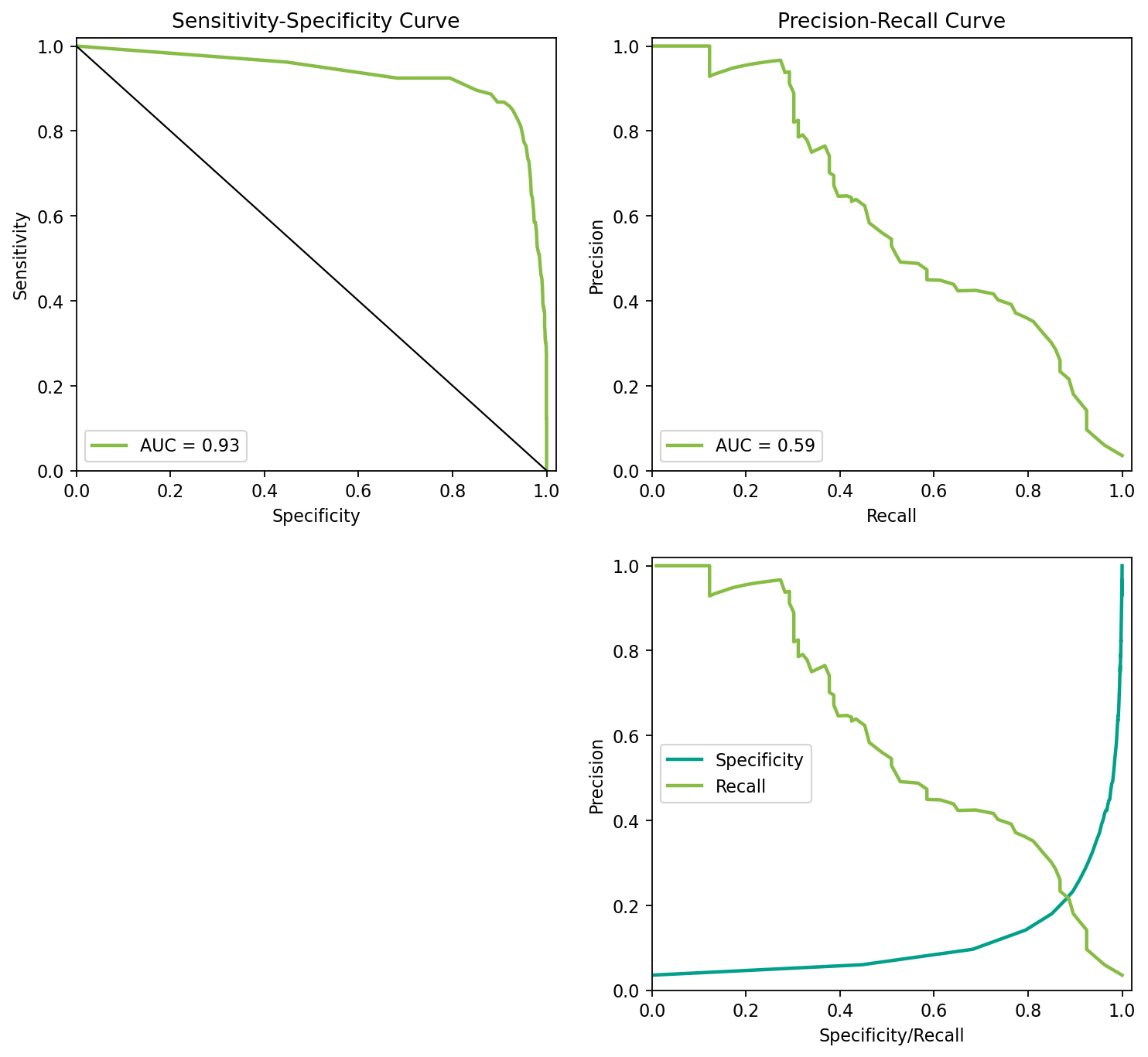
위에서 언급한 클래스 불균형의 예들: 이상치 탐지, 희귀 질병 진단 등에서는 precision & recall이 더 유용할 수 있음.
아래는 양성:음성 = 3:97인 경우의 예

code
from sklearn.datasets import make_classification
from sklearn.model_selection import train_test_split
from sklearn.ensemble import RandomForestClassifier
from sklearn.linear_model import LogisticRegression
from sklearn.metrics import roc_curve, auc, precision_recall_curve, average_precision_score

# Create an imbalanced dataset
X, y = make_classification(n_samples=10000, n_features=20, n_classes=2,
                           weights=[0.97, 0.03], random_state=42)

# Split the dataset into training and testing sets
X_train, X_test, y_train, y_test = train_test_split(X, y, test_size=0.3, random_state=42)

# Train a random forest classifier
clf = RandomForestClassifier(n_estimators=100, random_state=42)
clf.fit(X_train, y_train)

# Get the probability scores for the testing set
y_score = clf.predict_proba(X_test)[:, 1]

## 혹은 logistic regression
# lr = LogisticRegression()
# y_score = lr.predict_proba(X_test)[:, 1]

# Calculate the ROC curve
fpr, tpr, th = roc_curve(y_test, y_score)
spc = 1 - fpr
roc_auc = auc(fpr, tpr)

# Calculate the Precision-Recall curve
precision, recall, th2 = precision_recall_curve(y_test, y_score)
pr_auc = average_precision_score(y_test, y_score)

# Plot the ROC curve
plt.figure(figsize=(11, 10), dpi=80)
plt.subplot(2,2,1)
plt.plot(spc, tpr, color='#87bc45', lw=2, label='AUC = %0.2f' % roc_auc)
plt.plot([1, 0], [0, 1], color='k', lw=1, linestyle='-')
plt.xlim([0.0, 1.02])
plt.ylim([0.0, 1.02])
plt.xlabel('Specificity')
plt.ylabel('Sensitivity')
plt.title('Sensitivity-Specificity Curve')
plt.legend(loc="lower left")

# Plot the Precision-Recall curve
plt.subplot(2,2,2)
plt.plot(recall, precision, color='#87bc45', lw=2, label='AUC = %0.2f' % pr_auc)
plt.xlim([0.0, 1.02])
plt.ylim([0.0, 1.02])
plt.xlabel('Recall')
plt.ylabel('Precision')
plt.title('Precision-Recall Curve')
plt.legend(loc="lower left")

df1 = pd.DataFrame({"fpr": fpr, "tpr": tpr, "spc": spc, "th": th})
df2 = pd.DataFrame({"precision": precision, "recall": recall, "th": np.append(th2, 1)})
df_merge = df1.merge(df2)

plt.subplot(2,2,4)
plt.plot(df_merge["spc"], df_merge["precision"], color='#00A08A', lw=2)
plt.plot(df_merge["recall"], df_merge["precision"], color='#87bc45', lw=2)
plt.xlim([0.0, 1.02])
plt.ylim([0.0, 1.02])
plt.ylabel('Precision')
plt.xlabel('Specificity/Recall')
plt.legend(["Specificity", "Recall"])

plt.show()

Classifier의 전체적 성능에 대한 지표

ROC curve:

  • AUC: Area Under the Curve = Concordance Index
    • 각 specificity값에 대한 sensitivity의 합; 모형(classifier) 대한 전반적 평가
    • 0.5: random guess, 1: perfect prediction
  • Concordance Index(c-index): 모든 서로 다른 클래스의 Y쌍, 예를 들어 \((0_i, 1_j)\)에 대해서 해당하는 예측된 확률의 크기가 \(p_i < p_j\) 인 비율, 즉 순서가 맞는(concordance) 비율


위 blowdown 데이터셋 대한 모형의 AUC, concordance index 계산

Code
from sklearn.metrics import roc_auc_score, auc

roc_auc = roc_auc_score(test_pred.y, test_pred.pred_prob)
print(f"AUC: {roc_auc:.2f}")  # 또는 auc(fpr, tpr)

AUC: 0.81

Code
def concordance(y, pred_prob):
    concord = 0
    total = 0

    test_pred = pd.DataFrame({"y": y, "pred_prob": pred_prob})
    for idx, case in test_pred.iterrows():
        other_cases = test_pred[test_pred.index != idx]

        # 같은 케이스 제외
        df = other_cases[case["y"] != other_cases["y"]]

        concord += (
            (case["y"] - df["y"] > 0) == (case["pred_prob"] - df["pred_prob"] > 0)
        ).sum()
        total += len(df)

    return concord / total

print(f"Concordance index: {concordance(test_pred.y, test_pred.pred_prob):.2f}")

Concordance index: 0.81

Precision-recall:

  • Average precision: the area under the precision-recall curve
Code
from sklearn.metrics import average_precision_score

average_precision = average_precision_score(test_pred.y, test_pred.pred_prob)
print(f"Average Precision: {average_precision:.2f}")

Average Precision: 0.68


The classification report in scikit-learn
Thershold: 0.4인 경우,

code
from sklearn.metrics import classification_report, recall_score

threshold = .4
pred_class = test_pred["pred_prob"] >= threshold
print(classification_report(test_pred["y"], pred_class))
              precision    recall  f1-score   support

           0       0.86      0.82      0.84       222
           1       0.66      0.73      0.69       108

    accuracy                           0.79       330
   macro avg       0.76      0.77      0.77       330
weighted avg       0.80      0.79      0.79       330
Specificity

위 표에서 specificity는 음성(0)을 기준으로 보면 됨: 즉, 0을 양성으로 봤을 때의 recall값

  • Secificity for positive(1): recall for negative(0): 0.82

따라서, macro avg of recall의 의미는 sensitivity(0.73)와 specificity(0.82)의 평균: 0.77
weighted avg는 관측값(support)만큼 가중치를 적용한 평균

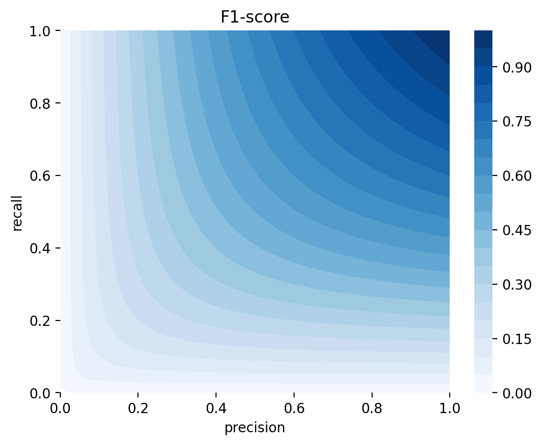
  • F1-score = \(\displaystyle \left(\frac{\text{precision}^{-1} + \text{recall}^{-1}}{2}\right)^{-1}\)
    • Precision과 recall의 조화평균
    • 보수적인 지표임. 즉, precision과 recall 중 하나라도 낮으면 F1-score도 낮아짐

종합: 모형평가

1. Classifier로서 전반적인 모형의 성능 vs. 2. 특정 임계치에서의 모형의 성능 vs. 3. 확률모형

  1. Classifier로서 전반적인 모형의 성능을 평가: AUC 등
  2. 비용을 고려한 특정 임계치에서의 모형의 성능
    • 잘못된 예측에 대한 비용이 다르다면, 임계치를 조정하여 기대 손실(Expected Loss)을 줄일 수 있음
    • 다음 두 가지 케이스를 보면,
폭우/태풍의 예측 문제

폭우 예측에서 농가의 경제적 손실을 손실(loss)로 가정하면:

  • Costs: 농작물 피해, 시설물 피해, 펜스 설치비, 노동력 투입 비용 등
  • Benefits: 농작물 수확 및 판매 수익

거짓 음성(False Negative, “폭우 없음”으로 예측했으나 실제로 폭우 발생)을 낮춰야 하는 경우

  • 폭우 발생 시 피해 규모가 매우 큰 경우
  • 예방 비용보다 피해 비용이 훨씬 큰 경우
  • 예:
    • 수확 직전 과수원(사과, 배, 복숭아 등)
    • 비닐하우스 시설이 폭우에 취약한 농가
    • 침수 시 작물 전체를 잃을 위험이 있는 농가
  • 이러한 경우에는 다소 과도하게 경보를 발령하더라도 큰 피해를 예방하는 것이 경제적으로 유리함

거짓 양성(False Positive, “폭우 발생”으로 예측했으나 실제로 폭우 미발생)을 낮춰야 하는 경우

  • 예방 조치 비용이 매우 큰 경우
  • 실제 폭우가 발생하더라도 피해 규모가 상대적으로 제한적인 경우
  • 예:
    • 폭우 대비를 위해 대규모 인력과 장비를 동원해야 하는 농가
    • 조기 수확 시 상품 가치가 크게 하락하는 고급 과일 농가
    • 배수 시설이나 보호 시설이 잘 갖추어져 있어 폭우 피해가 비교적 작은 농가
  • 이러한 경우에는 불필요한 대응 비용을 줄이기 위해 보다 높은 확률에서만 경보를 발령하는 것이 경제적으로 유리함

정리하면,

  • 폭우 피해 비용 > 예방 비용 → 거짓 음성을 줄이는 방향으로 임계치 조정
  • 예방 비용 > 폭우 피해 비용 → 거짓 양성을 줄이는 방향으로 임계치 조정
와인 품질 예측 문제

와인 셀러가 와인의 화학적 성분을 이용하여 품질을 예측하는 모형을 구축하는 경우,

  • 양성(Positive): 고품질 와인
  • 음성(Negative): 저품질 와인

Costs:

  • 거짓 음성(False Negative): 실제로는 고품질 와인인데 저품질로 분류
    • 프리미엄 가격을 받지 못함
    • 고품질 와인을 저가에 판매하여 수익 손실 발생
  • 거짓 양성(False Positive): 실제로는 저품질 와인인데 고품질로 분류
    • 고객 만족도 저하
    • 와인 평론가 및 소비자의 신뢰 상실
    • 브랜드 가치 하락
    • 장기적인 매출 감소 가능성

Benefits:

  • 고품질 와인을 정확히 고품질로 분류
    • 프리미엄 가격 책정 가능
    • 수익 증가
  • 저품질 와인을 정확히 저품질로 분류
    • 품질에 대한 신뢰 유지
    • 브랜드 이미지 보호

거짓 음성(False Negative)을 낮춰야 하는 경우
즉, 실제 고품질 와인을 저품질로 분류하는 것을 최소화해야 하는 경우

  • 예:
    • 신생 와이너리
    • 영세 와이너리
    • 브랜드 인지도가 낮은 생산자
  • 이들은 브랜드 가치보다 단기적인 현금 흐름과 수익 확보가 더 중요할 수 있음.
  • 따라서 일부 저품질 와인이 고품질로 분류될 위험을 감수하더라도, 실제 고품질 와인을 놓치지 않는 것이 중요함.
  • 즉, “좋은 와인을 싸게 파는 손실”을 최소화하는 전략

거짓 양성(False Positive)을 낮춰야 하는 경우
즉, 실제 저품질 와인을 고품질로 분류하는 것을 최소화해야 하는 경우

  • 예:
    • 프리미엄 와이너리
    • 고급 브랜드 이미지를 가진 생산자
    • 오랜 기간 품질로 명성을 구축한 와이너리
  • 이들은 한 번의 품질 실수가 브랜드 신뢰에 큰 타격을 줄 수 있음.
  • 따라서 일부 고품질 와인이 저품질로 분류되어 수익을 놓치더라도, 저품질 와인이 프리미엄 제품으로 판매되는 상황은 최대한 방지하려 함.
  • 즉, “수익 손실보다 브랜드 가치 보호”가 더 중요한 전략

정리하면,

  • 고품질 와인을 놓쳐 발생하는 수익 손실 > 저품질 와인을 고품질로 분류하여 발생하는 평판 손실 → 거짓 음성(False Negative)을 줄이는 방향으로 임계치 조정
  • 저품질 와인을 고품질로 분류하여 발생하는 평판 손실 > 고품질 와인을 놓쳐 발생하는 수익 손실 → 거짓 양성(False Positive)을 줄이는 방향으로 임계치 조정
  1. 확률을 정확히 예측하는 모형의 추구
  • 단순히 “양성/음성”을 예측하는 것이 아니라, 사건이 발생할 확률을 정확하게 추정하는 것을 목표로 함
  • 단일 확률값뿐 아니라 그 확률값의 분포 전체(Bayesian 접근)를 제공하여 예측값의 불확실성까지 전달함
  • 모형은 의사결정을 내리는 것이 아니라, 의사결정에 필요한 정보를 제공하는 역할을 수행함
  • 실제 decision maker는 당사자/소비자
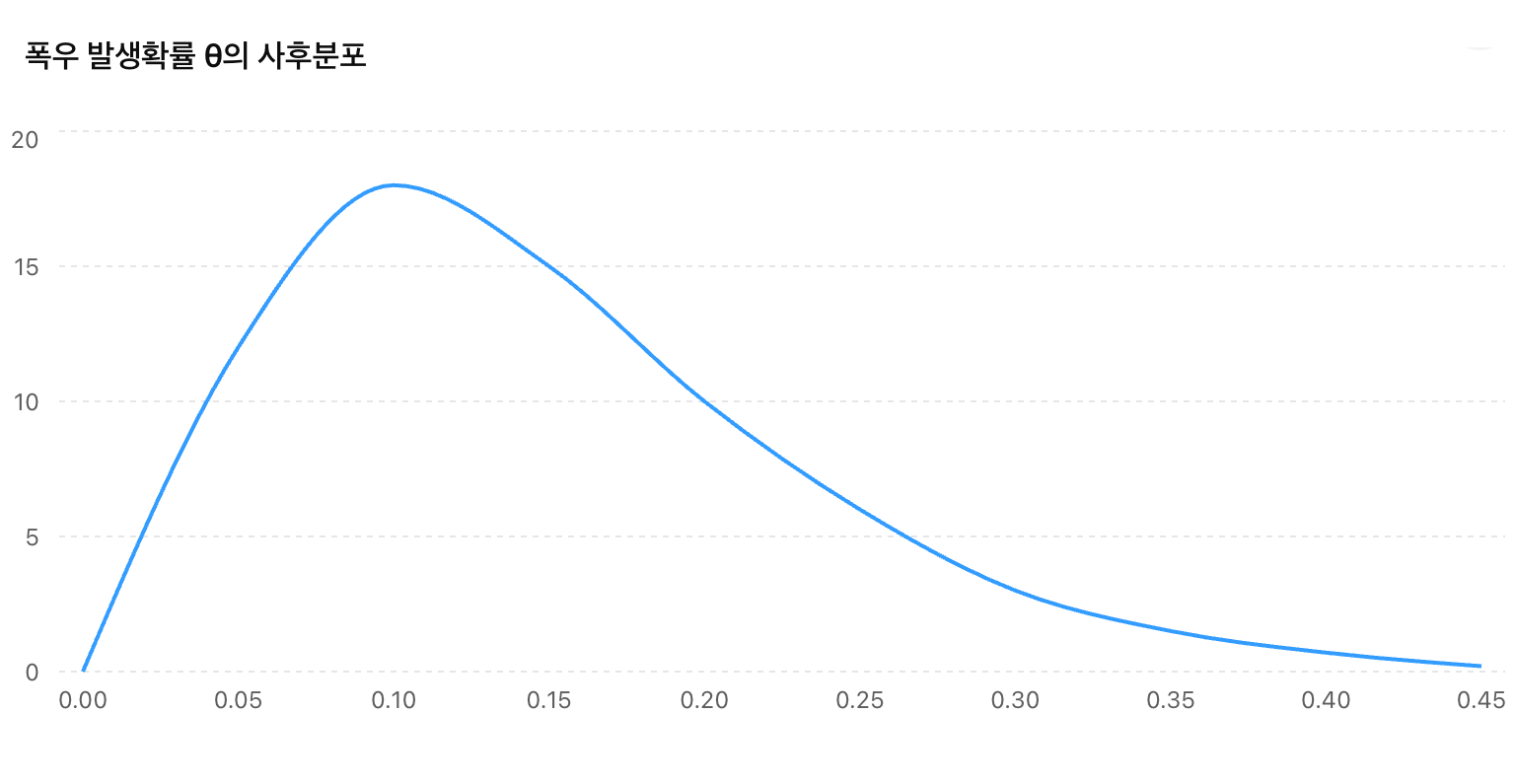
Bayesian적 접근

예를 들어, 폭우 예측 문제에서 폭우 발생확률 \(p\)의 사후분포를 다음과 같이 얻을 수 있음.
즉, 폭우가 올 (최선의) 확률값 하나를 얻는 것이 아니고, 폭우가 올 모든 확률값의 가능성의 분포를 얻게 됨.

Bayesian posterior distribution

가령, 이 분포를 이용해 모든 가능한 \(p\)에 대한 기대 손실(expected loss)들의 기대값으로 총 손실을 계산할 수 있음

Frequentist 접근에서는 종종 “가장 가능성이 높은 결과”에 주목하지만,
Bayesian 접근에서는 예측분포 전체를 이용하여 기대손실(Expected Loss)을 계산하고 의사결정을 수행

Decision Boundary

앞선, Log odds(logit):   \(\displaystyle log\left(\frac{\hat{p}}{1 - \hat{p}}\right) = b_0 + b_1 \cdot X\)
예측변수가 2개라면,

Log odds(logit):   \(\displaystyle log\left(\frac{\hat{p}}{1 - \hat{p}}\right) = b_0 + b_1 \cdot X_1 + b_2 \cdot X_2\)

또는 \(\displaystyle \hat p = \sigma(b_0 + b_1 \cdot X_1 + b_2 \cdot X_2)\),   \(\displaystyle \sigma := \frac{1}{1 + e^{-x}}\)

  • 왼편의 logit 함수(또는 sigmoid 함수)는 증가함수이므로, threshold를 정하면 선형 결정 경계(decision boundary)가 나타남: hyperplane
  • 비선형 함수로 모형을 세우면, decision boundary가 비선형으로 나타남.
    • 예를 들어, \(b_0 + b_1 \cdot X + b_2 \cdot X^2\) 등

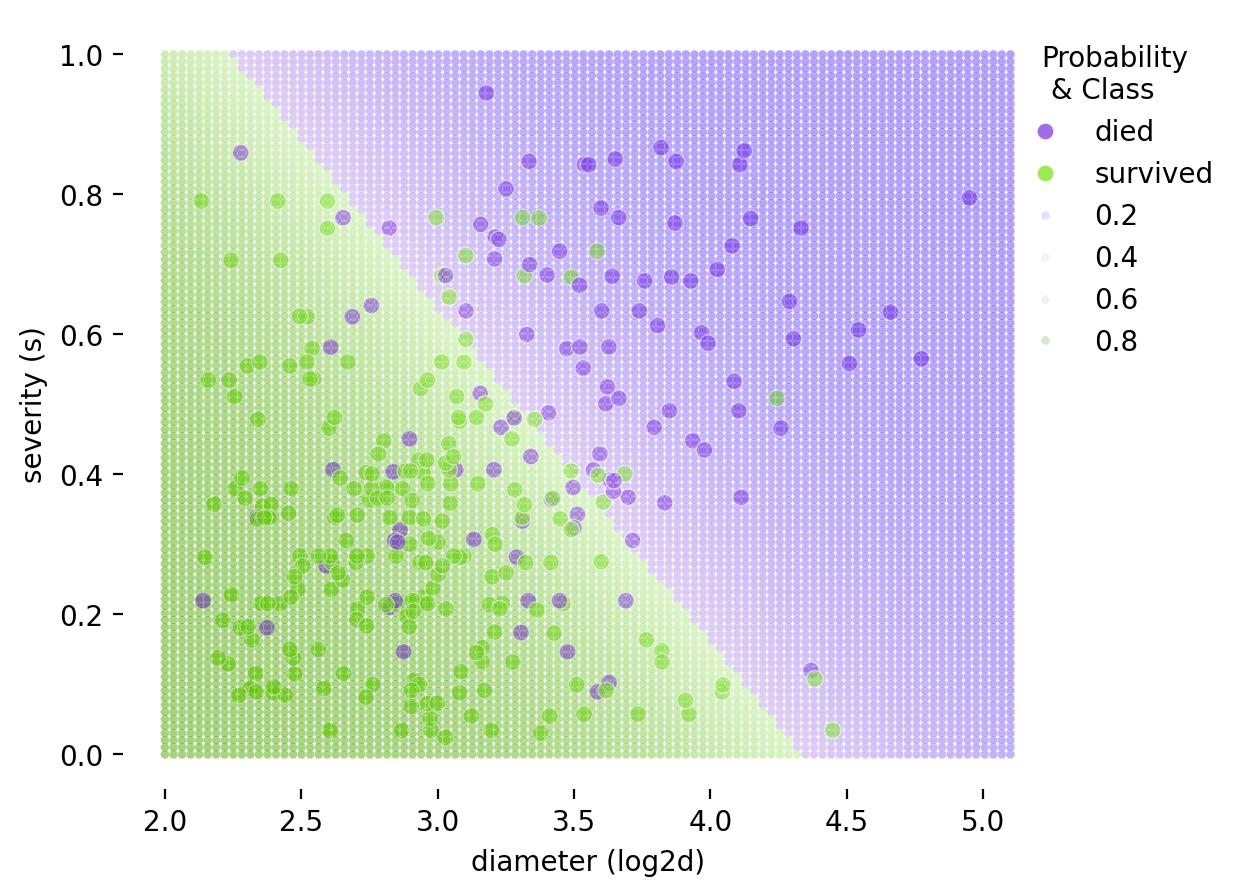
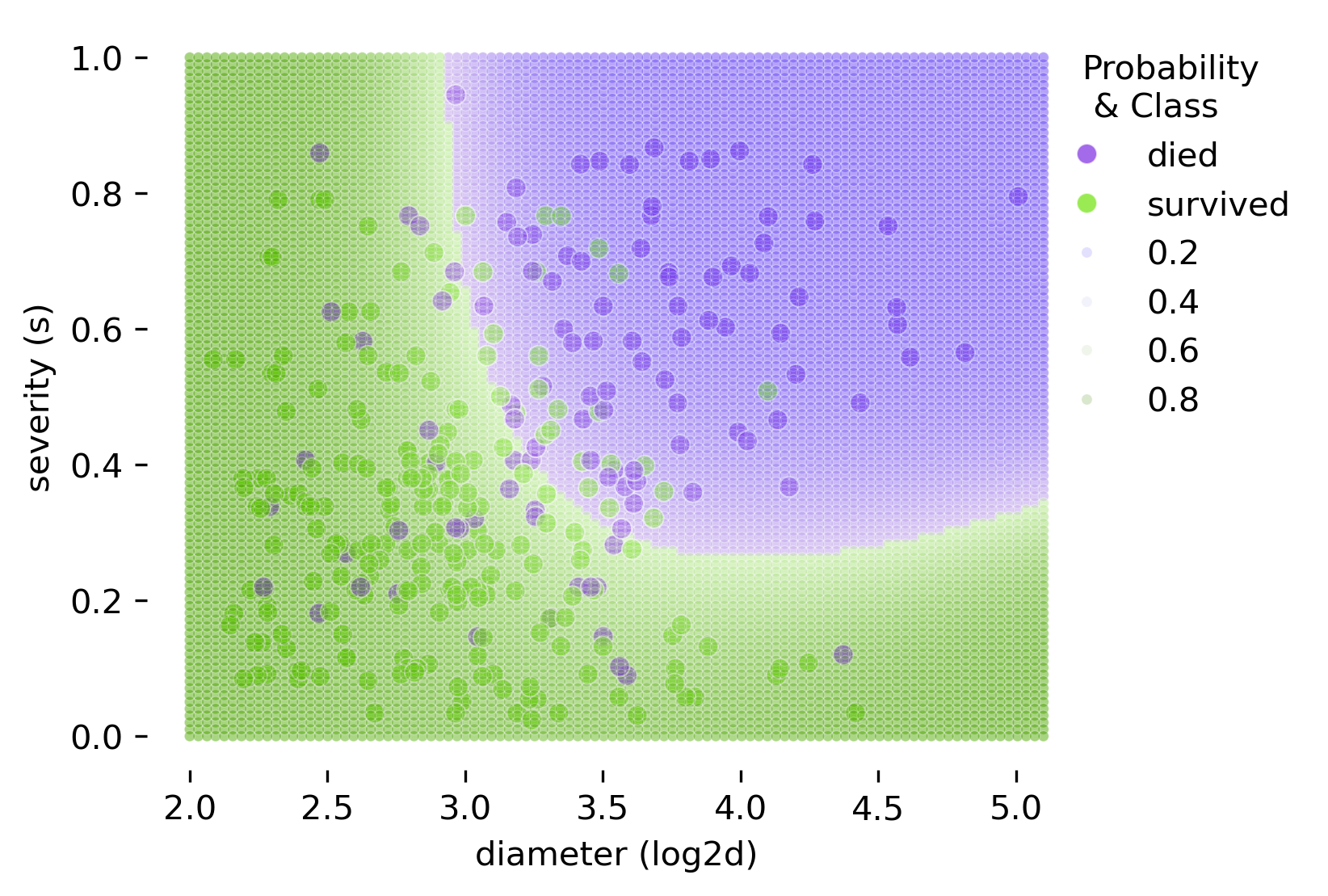
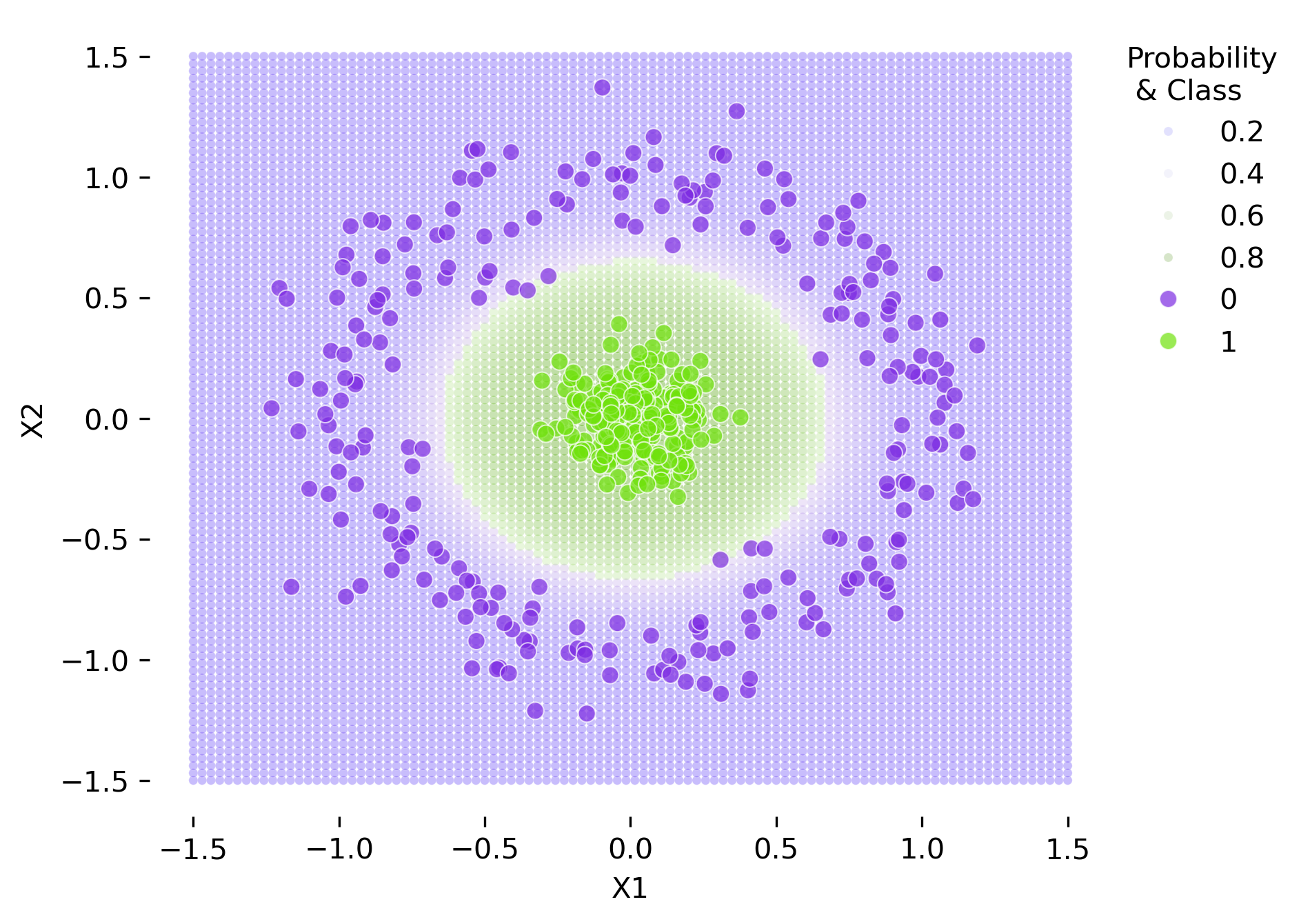
밑은 두 예측변수 \(X_1= log2d\) (diameter)와 \(X_2=s\) (severity)로 나무가 쓰러질지 여부를 선형함수로 만들었을 때의 decision boundary (threshold=0.5)
즉, Log odds(logit):   \(\displaystyle log\left(\frac{\hat{p}}{1 - \hat{p}}\right) = b_0 + b_1 \cdot X_1 + b_2 \cdot X_2\)

BodyM Dataset

AWS: BodyM Dataset

  • 2,779명 대상으로 8,324장의 정면 및 측면 실루엣 사진과 키, 몸무게, 그리고 14가지 신체 측정치 제공
  • 인종 분포: 백인 40%, 아시아인 30%, 흑인/아프리카계 미국인 14%, 아메리카 원주민 또는 알래스카 원주민 1%, 기타 15%(히스패닉 15%)
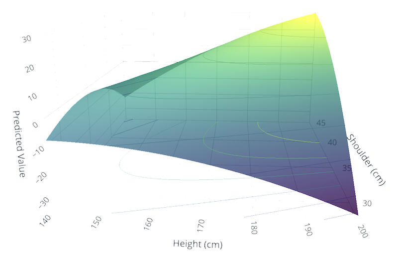
\(Y\) = 성별,
\(X_1\) = 키(height), \(X_2\) = 어깨 너비(shoulder-breath)에 대한 2차항을 포함한 선형함수로 모형을 세웠을 때의 decision boundary

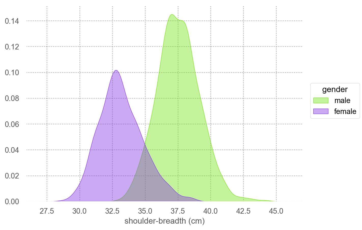
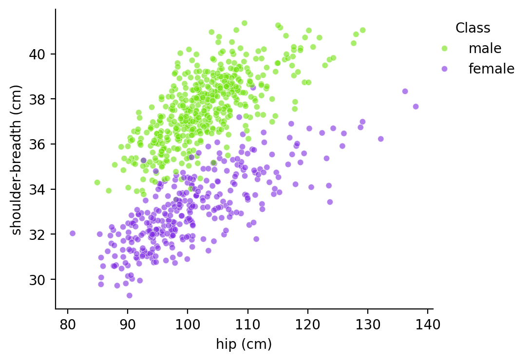
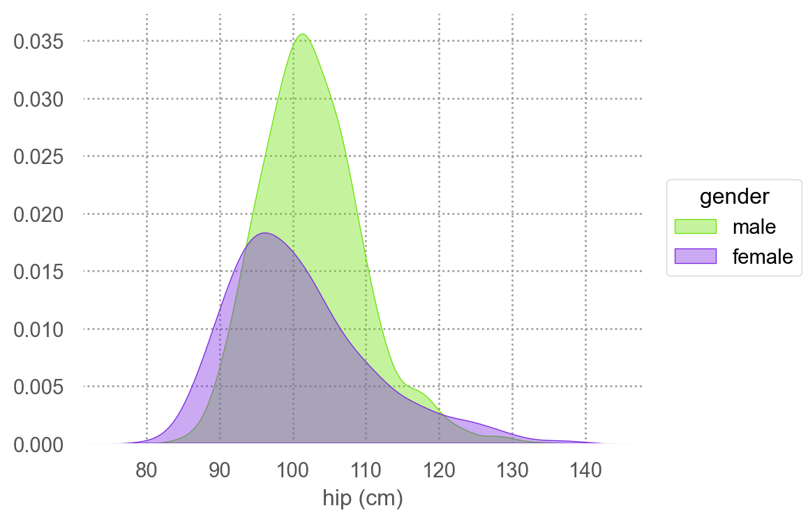
Shoulder와 hip 정보로 분류하다면?

Basis Functions

기저 함수

관측치(input vector) \(\mathbf{x}\)에 대해, basis function \(\phi(\mathbf{x})\)를 사용하여, 비선형 모형을 선형모형의 형태로 변환(파라미터에 대한 선형)

\[\mathbf{y} = b_0 + b_1 \cdot \phi_1(\mathbf{x}) + b_2 \cdot \phi_2(\mathbf{x}) + ... + b_n \cdot \phi_{m-1}(\mathbf{x})\]

예를 들어, 두 예측변수의 관측치 \(\mathbf{x} = (x_1, x_2) = (log2d, s)\) (각각 diameter와 severity)에 대해서 모든 2차항을 추가한다면

\[\phi_i(\mathbf{x}): \mathbb{R}^2 \to \mathbb{R}\]

where \(\phi_1(\mathbf{x}) = x_1, ~ \phi_2(\mathbf{x}) = x_2, ~ \phi_3(\mathbf{x}) = x_1^2, ~ \phi_4(\mathbf{x}) = x_1 \cdot x_2, ~ \phi_5(\mathbf{x}) = x_2^2\)

  • 즉, 5개의 예측 변수가 생성: \(x_1, x_2, x_1^2, ~ x_1 \cdot x_2, ~x_2^2\)
  • 이는 2차원 예측변수 공간을 5차원으로 확장하는 것과 같음: \((x_1, x_2) \rightarrow (\phi_1, \phi_2, \phi_3, \phi_4, \phi_5)\)
  • 이는 Kernel trick과 유사함: 고차원으로 변환하여 선형모형을 적용하는 것
  • Feature engineering의 일종임. Deep learning에서는 연구자가 직접 만들기보다는 모형이 학습할 수 있도록 함.
code
# 2차식을 추가
from sklearn.preprocessing import PolynomialFeatures
from sklearn.linear_model import LogisticRegression
from ISLP import confusion_table
from sklearn.metrics import accuracy_score

poly = PolynomialFeatures(degree=2)
X_train_poly = poly.fit_transform(X_train)
X_test_poly = poly.transform(X_test)

lr_poly = LogisticRegression(penalty=None, max_iter=1000)
lr_blowsdn_poly = lr_poly.fit(X_train_poly, y_train)

test_pred = X_test.assign(
    y=y_test,
    pred_prob=lr_blowsdn_poly.predict_proba(X_test_poly)[:, 1],  # 확률값
    pred_class=lr_blowsdn_poly.predict(X_test_poly),  # 클래스
)

# cutoff = 0.5
cm = confusion_table(test_pred["pred_class"], test_pred["y"])
score = accuracy_score(test_pred["y"], test_pred["pred_class"])
Figure 1: Logistic Regression Decision Boundary with Kernel Tricks
(a) \(\phi: (x_1, x_2) \rightarrow (x_1, x_2, x_1^2, x_1 x_2, x_2^2) \in \mathbb{R^5}\)
(b) \(\phi: (x_1, x_2) \rightarrow (x_1, x_2, x_1^2 + x_2^2) \in \mathbb{R^3}\)

선형모형은 basis function을 고려하면 간단한 neural network(신경망)으로 볼 수 있음.

자주 사용되는 basis function

  • Polynomial basis: \(\phi_i(x) = x^i\)
  • Gaussian (Radial) basis: \(\displaystyle \phi_i(\mathbf{x}) = \exp\left(-\frac{||\mathbf{x} - \mu_i||^2}{2 s^2}\right)\)
  • Sigmoidal basis: \(\displaystyle \phi_i(\mathbf{x}) = \sigma\left(\frac{||\mathbf{x} - \mu_i||}{s}\right)\), \(\displaystyle \sigma(x) = \frac{1}{1 + e^{-x}}\)

다른 모형에서도 유연하게 비슷한 아이디어를 적용할 수 있음.

  • 가령, KNN에서 이웃하는 데이터들 간의 거리를 고려해서 확률을 계산할 수 있음.
  • 즉, Gaussian의 분포에 비례하여 근접한 이웃에 더 큰 가중치를 부여함.

KNN with Gaussian kernel
def gaussian_kernel(distances, sigma=1):
  """Calculates Gaussian kernel weights."""
  return np.exp(-distances**2 / (2 * sigma**2))

# Create KNN classifier with custom weights
knn_gaussin = KNeighborsClassifier(n_neighbors=10, weights=lambda x: gaussian_kernel(x, sigma=1))

Neural Network/Deep Learning

  • 앞서 Gaussian basis (radial basis) function (RBF)과 같은 방식으로 비선형 모형 변환이 유용하나, 계산량이 많고, 과적합을 방지하기 위한 조심스러운 정규화가 필요함.
  • 또는, Support Vector Machine (SVM)도 비슷하게 basis function을 이용해 비선형 모형을 만드나, 확률적 출력을 제공하지 않고 다중 클래스의 일반화가 어려움.
  • RBF 및 SVM 같은 모델은 최근에는 deep learning에 의해 대체되고 있음.
    • 대규모 데이터셋을 효과적으로 활용 가능.
    • 깊은 계층 구조의 표현을 학습하여 복잡한 예측 문제에서 높은 정확도 달성.

FIGURE 10.1. Neural network with a single hidden layer. The hidden layer computes activations \(A_k = h_k(X)\) that are nonlinear transformations of linear combinations of the inputs \(X1, X2, . . . , Xp\). Hence these \(A_k\) are not directly observed. The functions \(h_k(\cdot)\) are not fixed in advance, but are learned during the training of the network. The output layer is a linear model that uses these activations \(A_k\) as inputs, resulting in a function \(f(X)\).


FIGURE 10.2. Activation functions. The piecewise-linear ReLU function is popular for its efficiency and computability. We have scaled it down by a factor of five for ease of comparison.

  • Hidden layers: \(A_k = g(w_{k0} + w_{k1}X_1 + w_{k2}X_2 + w_{k3}X_3 + w_{k4}X_4)\)
    • \(g\)는 activation function으로 logistic에서처럼 sigmoid나 현대적으로는 ReLU를 사용
  • 각 \(A_k\)가 1에 가까우면 firing, 0에 가까우면 silent한다고 마치 뇌의 뉴런이 신호가 전달되는 것에 비유
  • \(Y(X) = \beta_0 + \beta_1 A_1 + \beta_2 A_2 + \cdots + \beta_5 A_5\)

The handwritten digit recognition example

  • 1980년대 후반 숫자를 인식하는 문제가 신경망 기술의 발전에 큰 촉매로 작용했음.
  • 신경망의 구조의 개선을 거쳐 인간 수준의 성능을 달성하는데 30년 이상 걸렸음.

아래 28x28 pixels의 음영을 나타내는 0~255(8bit) 값을 입력값으로 받음.

  • 60,000개의 training set을 이용하여 학습
  • 인풋 레이어의 유닛(unit)의 수: 28x28 = 784개 (예측변수의 수)
  • 각각의 hidden layer의 유닛의 수는 256개, 128개
  • 총 파라미터의 수는 235,146개; 예측변수보다 월등히 많음
  • 한편 multinomial logistic으로 필요한 파라미터의 수는 785x9 = 7,065개

Source: 3blue1brown

 Source: An Introduction to Statistical Learning (2e)

Convolutional Deep Belief Networks: Hierarchical Representations

Source: p.301, 293, Deep Learning: Foundations and Concepts by Bishop, C. M. & Bishop, H

Figure 2. The first layer bases (top) and the second layer bases (bottom) learned from natural images. Each second layer basis (filter) was visualized as a weighted linear combination of the first layer bases.

Figure 2. The first layer bases (top) and the second layer bases (bottom) learned from natural images. Each second layer basis (filter) was visualized as a weighted linear combination of the first layer bases.

Figure 3. Columns 1-4: the second layer bases (top) and the third layer bases (bottom) learned from specific object categories. Column 5: the second layer bases (top) and the third layer bases (bottom) learned from a mixture of four object categories (faces, cars, airplanes, motorbikes).

Figure 3. Columns 1-4: the second layer bases (top) and the third layer bases (bottom) learned from specific object categories. Column 5: the second layer bases (top) and the third layer bases (bottom) learned from a mixture of four object categories (faces, cars, airplanes, motorbikes).

Source: Convolutional Deep Belief Networks

Google Neural Network Playground

Multiclass (K > 2)

Multinomial logistic regression

클래스 \(C_k\)에 속할 확률을 예측하는 모형: Base 클래스를 기준으로 나머지 클래스에 대한 확률을 예측
Binary 경우에서의 확률 \(\displaystyle P(Y=1|X=x) = \frac{1}{1+e^{-(b_0 + b_1 \cdot x)}}=\frac{e^{b_0 + b_1 \cdot x}}{1 + e^{b_0 + b_1 \cdot x}}\)을 다음과 같이 확장할 수 있음.

  • \(\displaystyle P(Y=C_k|X=x) = \frac{e^{\beta_{k0} + \beta_{k1} \cdot x}}{1 + \sum_{j=1}^{K-1} e^{\beta_{j0} + \beta_{j1} \cdot x}}, ~~ k = 1, 2, ..., K-1\)
  • \(k=K\) (Base 클래스)의 경우 \(\displaystyle P(Y=C_K|X=x) = \frac{1}{1 + \sum_{j=1}^{K-1} e^{\beta_{j0} + \beta_{j1} \cdot x}}\)

이 때, 마지막 클래스 \(C_K\)에 대한 클래스 \(C_k\)의 비율은 다음과 같이 나타남.

\(\displaystyle log\left(\frac{P(Y=C_k|X=x)}{P(Y=C_K|X=x)}\right) = \beta_{k0} + \beta_{k1} \cdot x\)

이는 binary경우 \(log(odds)\) 인 \(\displaystyle log\left(\frac{\hat{p}}{1 - \hat{p}}\right) = b_0 + b_1 \cdot x\)의 확장으로 볼 수 있음.

Note

Machine learning에서는 주로 base 클래스 없이 모든 클래스에 대한 확률을 예측:

Softmax coding: \(\displaystyle P(Y=C_k|X=x) = \frac{e^{\beta_{k0} + \beta_{k1} \cdot x}}{\sum_{j=1}^{K} e^{\beta_{j0} + \beta_{j1} \cdot x}}\)

두 클래스 \(C_k\)와 \(C_{k'}\)의 사이의 확률의 비율은

\(\displaystyle log\left(\frac{P(Y=C_k|X=x)}{P(Y=C_{k'}|X=x)}\right) = (\beta_{k0} - \beta_{k'0}) + (\beta_{k1} - \beta_{k'1}) \cdot x\)

Blowdown data

가령, 나무의 종(9 species)을 분류하는 문제를 생각해보면,
나무의 두께(log2d), 쓰러졌는지 여부(y), 피해 심각도(s)로 9개의 종에 대한 확률을 예측하는 모형을 만들 수 있음.

Load data
# Multinomial logistic regression
blowdown = pd.read_csv('data/blowdown2.csv')
X = blowdown.drop(columns=["spp", "d"])
y = blowdown["spp"]  # classify the species
blowdown
d s y spp log2d
0 9.00 0.02 0 balsam fir 3.17
1 14.00 0.02 0 balsam fir 3.81
2 18.00 0.02 0 balsam fir 4.17
... ... ... ... ... ...
3663 19.00 0.98 1 jackpine 4.25
3664 37.00 0.98 1 black ash 5.21
3665 48.00 0.98 1 black ash 5.58

3666 rows × 5 columns

# split the data into training and test sets
X_train, X_test, y_train, y_test = train_test_split(X, y, test_size=0.5, random_state=0, stratify=y)

lr = LogisticRegression(max_iter=1000)
lr.fit(X_train, y_train);
Predicted probability
pd.options.display.max_columns = 15

# predicted probability
test_pred_prob = pd.DataFrame(lr.predict_proba(X_test), columns=lr.classes_)
pd.concat(
    [X_test.assign(target=y_test).reset_index(drop=True), test_pred_prob], axis=1
) # 데이터셋 병합
s y log2d target aspen balsam fir black ash black spruce cedar jackpine paper birch red maple red pine
0 0.61 1 4.58 paper birch 0.29 0.00 0.02 0.04 0.24 0.02 0.33 0.01 0.04
1 0.26 0 4.32 cedar 0.14 0.02 0.01 0.05 0.20 0.26 0.11 0.04 0.18
2 0.86 1 5.17 aspen 0.42 0.00 0.09 0.01 0.10 0.01 0.34 0.00 0.02
... ... ... ... ... ... ... ... ... ... ... ... ... ...
1830 0.09 0 3.70 cedar 0.05 0.05 0.00 0.13 0.25 0.22 0.05 0.05 0.20
1831 0.41 1 3.32 black spruce 0.05 0.01 0.00 0.33 0.44 0.02 0.06 0.02 0.06
1832 0.20 0 3.00 cedar 0.01 0.05 0.00 0.31 0.24 0.12 0.01 0.06 0.21

1833 rows × 13 columns

Predicted class
# prediction
test_pred = X_test.assign(
    target=y_test,
    pred_class=lr.predict(X_test),
    pred_prob=lr.predict_proba(X_test).max(axis=1),
)
test_pred
s y log2d target pred_class pred_prob
2811 0.61 1 4.58 paper birch paper birch 0.33
1105 0.26 0 4.32 cedar jackpine 0.26
3566 0.86 1 5.17 aspen aspen 0.42
... ... ... ... ... ... ...
255 0.09 0 3.70 cedar cedar 0.25
1934 0.41 1 3.32 black spruce cedar 0.44
816 0.20 0 3.00 cedar black spruce 0.31

1833 rows × 6 columns

# confusion matrix
confusion_table(test_pred["pred_class"], test_pred["y"])
Truth aspen balsam fir black ash black spruce cedar jackpine paper birch red maple red pine
Predicted
aspen 38 0 6 0 7 12 30 0 7
balsam fir 0 0 0 0 0 0 0 0 0
black ash 2 0 1 0 0 0 0 0 0
black spruce 8 19 0 189 88 41 0 13 74
cedar 63 7 0 111 278 46 79 25 76
jackpine 21 4 0 8 47 45 24 11 28
paper birch 80 0 18 4 27 11 114 1 11
red maple 0 0 0 0 0 0 0 0 0
red pine 6 7 0 17 38 23 4 12 52

Precision, Recall: one-versus-all(rest)
해당 클래스를 positive로 두고 나머지 클래스를 negative로 두어, 각 클래스에 대한 precision과 recall을 계산

# classification report: one-versus-all
print(classification_report(test_pred["y"], test_pred["pred_class"]))
              precision    recall  f1-score   support

       aspen       0.38      0.17      0.24       218
  balsam fir       0.00      0.00      0.00        37
   black ash       0.33      0.04      0.07        25
black spruce       0.44      0.57      0.50       329
       cedar       0.41      0.57      0.48       485
    jackpine       0.24      0.25      0.25       178
 paper birch       0.43      0.45      0.44       251
   red maple       0.00      0.00      0.00        62
    red pine       0.33      0.21      0.26       248

    accuracy                           0.39      1833
   macro avg       0.28      0.25      0.25      1833
weighted avg       0.36      0.39      0.36      1833
# accuracy
print(accuracy_score(test_pred["y"], test_pred["pred_class"]))
0.3911620294599018

MNIST digits data

Load data
import tensorflow as tf

# Load the MNIST dataset
(X_train, y_train), (X_test, y_test) = tf.keras.datasets.mnist.load_data()

# randomly select a subset of the data
np.random.seed(123)

n1, n2 = 2000, 2000  # 2000 training and 2000 test samples

idx1 = np.random.randint(0, 60000, n1)
idx2 = np.random.randint(0, 10000, n2)

X_train_sub = X_train[idx1, :]
y_train_sub = y_train[idx1]
X_test_sub = X_test[idx2, :]
y_test_sub = y_test[idx2]

# Reshape the data
X_train_sub = X_train_sub.reshape(n1, 28 * 28)  # 2-dim array: (2000, 784)
X_test_sub = X_test_sub.reshape(n2, 28 * 28)
# Fit Logistic Regression with polynomial features
from sklearn.preprocessing import PolynomialFeatures

# Create polynomial features
poly = PolynomialFeatures(degree=2)
X_train_poly = poly.fit_transform(X_train_sub)
X_test_poly = poly.transform(X_test_sub)

# Fit the model
lr = LogisticRegression(max_iter=1000)
lr.fit(X_train_poly, y_train_sub)

# Prediction
y_pred_poly = lr.predict(X_test_poly)
Predicted probability
pd.options.display.max_columns = 15

# predicted probability
test_pred_prob = pd.DataFrame(lr.predict_proba(X_test_poly), columns=lr.classes_)
test_pred_prob["target"] = y_test_sub
test_pred_prob
0 1 2 3 4 5 6 7 8 9 target
0 0.01 0.00 0.00 0.00 0.00 0.98 0.00 0.00 0.02 0.00 8
1 0.00 0.00 0.00 0.00 1.00 0.00 0.00 0.00 0.00 0.00 4
2 0.00 0.00 0.00 0.00 0.00 0.00 0.00 1.00 0.00 0.00 7
... ... ... ... ... ... ... ... ... ... ... ...
1997 1.00 0.00 0.00 0.00 0.00 0.00 0.00 0.00 0.00 0.00 0
1998 1.00 0.00 0.00 0.00 0.00 0.00 0.00 0.00 0.00 0.00 0
1999 0.00 0.00 0.00 0.00 0.00 0.00 1.00 0.00 0.00 0.00 6

2000 rows × 11 columns

Confusion Matrix
from ISLP import confusion_table
confusion_table(y_pred_poly, y_test_sub)
Truth 0 1 2 3 4 5 6 7 8 9
Predicted
0 186 0 2 0 0 4 5 0 1 1
1 0 222 2 1 0 3 0 6 1 1
2 2 1 179 3 5 0 0 6 2 0
3 1 0 7 191 0 2 1 1 8 3
4 0 1 0 0 173 1 4 0 3 8
5 1 1 1 4 1 156 3 0 4 1
6 0 4 2 1 4 3 187 0 4 0
7 3 0 1 4 0 0 0 179 2 7
8 0 1 0 1 3 3 0 0 174 3
9 0 0 1 1 6 1 0 4 0 192
Classification Report
from sklearn.metrics import classification_report, accuracy_score

# accuracy
print("Predictive Accuracy:", accuracy_score(y_test_sub, y_pred_poly))

# classification report: one-versus-all
print("\nClassification Report:\n", classification_report(y_test_sub, y_pred_poly))
Predictive Accuracy: 0.9195

Classification Report:
               precision    recall  f1-score   support

           0       0.93      0.96      0.95       193
           1       0.94      0.97      0.95       230
           2       0.90      0.92      0.91       195
           3       0.89      0.93      0.91       206
           4       0.91      0.90      0.91       192
           5       0.91      0.90      0.90       173
           6       0.91      0.94      0.92       200
           7       0.91      0.91      0.91       196
           8       0.94      0.87      0.91       199
           9       0.94      0.89      0.91       216

    accuracy                           0.92      2000
   macro avg       0.92      0.92      0.92      2000
weighted avg       0.92      0.92      0.92      2000

Other Model Families

선형모델을 확장한 다양한 모델들이 존재

  • Robust linear models: 중심에서 먼 outlier에 대한 잔차의 영향을 줄여서 파라미터를 추정
  • Penalised linear models: 파라미터에 제한을 두어 estimation. 예를 들어, ridge regression, lasso regression
  • Generalised linear models (GLM): 예를 들어, logistic regression, Poisson regression
  • Generalised additive models (GAM): GLM을 더 확장하여 각 예측변수에 대해 smooth functions를 사용하여 nonlinear 관계를 모델링
    • \(g(E(Y | X)) = \beta_0 + f_1(X_1) + f_2(X_2) + f_3(X_1, X_2)\)
    • Basis functions도 그 일종임
    • Splines, loess, smoothing splines 등
K-Nearest Neighbors
Generative Models

This work © 2024 by Sungkyun Cho is licensed under CC BY-NC-SA 4.0